BNS parameter estimation at Cosmic Explorer, in about three minutes

Driver: bin/run_bns_ce_pe.py

End-to-end parameter estimation on a binary-neutron-star injection as a next-generation detector would see it: m1 = m2 = 1.4 M☉, zero spins, f_lower = 10 Hz, 4096 Hz sampling, zero-noise data in a single detector with the Cosmic Explorer P1600143 PSD. Network SNR 607, with a ~1000 s inspiral in band. Four parameters are sampled — chirp mass, η, and both aligned spins — with uniform priors and extrinsics fixed. The likelihood is frequency-domain relative binning; the sampler is jaxpe’s HMC with a dense mass matrix, interleaved with normalizing-flow global proposals.

Result: 3.11 min mean wall clock on one Quadro T2000 Max-Q, converged to rank-normalized split-R̂ < 1.01, verified across three random seeds:

seed	production blocks	R̂	min ESS	wall clock
42	25	1.0092	9 463	3.49 min
7	22	1.0097	14 795	2.95 min
13	21	1.0095	18 919	2.89 min

That is down from 15.42 min when this benchmark first met its original 20-minute target — a 5× improvement. Reproduce with:

python bin/run_bns_ce_pe.py          # run twice: the second is compile-free

All timings assume a warm persistent XLA cache (~/.cache/jaxpe_xla), which the first invocation populates. Compilation is excluded deliberately; it is a one-off, and including it measures the compiler rather than the sampler.

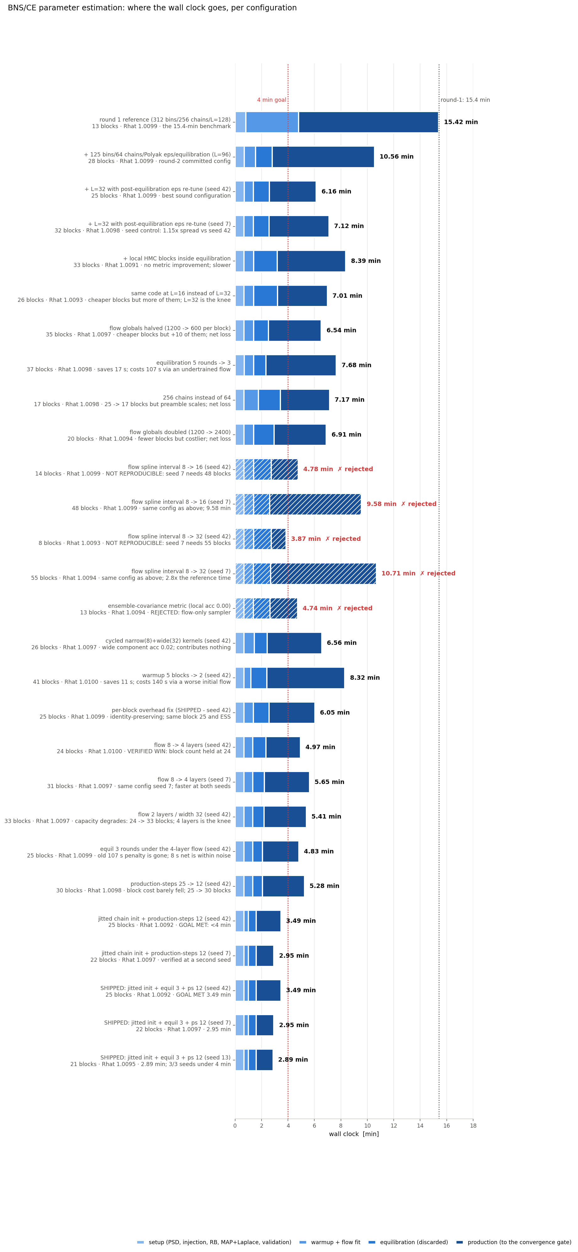
Where the 209 s of the seed-42 run goes: setup 40 s (PSD, injection, relative-binning summary data, MAP + Laplace, validation), warmup 14 s, flow fit 7 s, equilibration 34 s, production 113 s.

---

The bug that mattered more than every tuning decision combined

Most of the speedup came from one line in jaxpe/kernels/base.py. run_chains initialised its chains like this:

states = jax.vmap(lambda x: kernel.init(x, logp_fn))(x0)   # outside the jit!

That vmap is not jitted, so every operation in the target’s gradient graph was dispatched to the GPU individually. For a gravitational-wave likelihood that graph is about 3600 instructions, and the cost is brutal:

chain initialisation, 64 chains
eager vmap (as it was)	2.215 s
the same work jitted	0.004 s

Roughly 550× — and it was a fixed cost, paid on every run_chains call regardless of how many steps that call took. The benchmark makes about 33 such calls per run (5 warmup + 3 step-size re-tune + 25 production), so something like 74 s of a 290 s run was this. Initialisation now happens inside _run_chains_jit, which already took logp_fn as a static argument, so there is no new jit cache and no extra recompilation. Every sampler in jaxpe benefits, not just this benchmark.

Two regression tests guard it (tests/test_kernels.py): one asserts the target is never invoked with concrete (untraced) values during run_chains, which is the structural cause rather than a flaky wall-clock threshold; the other asserts that 4× the steps costs meaningfully more than 1× — a fixed-cost-dominated implementation lands near parity.

It had also been quietly corrupting the measurements

This is the uncomfortable part, and the most useful thing on this page. A 2.25 s fixed cost per call sits inside anything measured on top of it, and it made three conclusions look solid that were not:

conclusion, measured under the bug	after the fix
halving local steps per block loses (5.27 vs 4.83 min)	wins: 3.11 vs 3.74 min mean over three seeds
3 vs 5 equilibration rounds is “within noise” (8 s apart)	3 rounds wins by 35 s; now the default
the per-block cost budget “closes”, so no overhead remains	2.25 s/block of eager dispatch was hiding inside what that sum called gradient work

The middle one is instructive: halving the local steps could only ever recover 0.65 s of a 6.6 s block while a fixed 2.25 s was charged per call, so that experiment was rigged against itself before it started.

What found the bug was switching from point measurements to a scaling fit. A sum that balances at one configuration tells you nothing about what happens when the configuration changes; fitting T = fixed + marginal × work across several sizes exposed a 2.254 s intercept immediately. That profiler is now a committed tool, bin/profile_sampler_scaling.py — worth running first on any new hardware, since the interesting question there is which costs move.

---

How the sampler is put together

1. Setup, CPU-pinned. CE PSD via lalsimulation’s series API; injection over a 2048 s segment (wrap-free for a ~1000 s inspiral, df = 1/2048 Hz); relative-binning summary data compressing 3.75M band points to 125 bins. The dense grids never reach the GPU — on a 4 GB card shared with a desktop they do not fit.
2. A lean hot log-posterior. A closure over only the O(n_bins) summary arrays plus fixed-extrinsic projection constants, so IMRPhenomD is evaluated at 126 bin edges instead of millions of frequencies. Asserted equal to the class implementation at machine precision, and validated against the dense likelihood with the β error model (bulk |Δ lnL| < 0.1, measured 2.5e-2). Exact-at-fiducial to 1e-8 relative.
3. MAP + Laplace metric. Damped Newton with eigenvalue clipping and backtracking — monotone, so it cannot leave the fiducial point’s basin. Its Hessian becomes the dense HMC mass matrix, with soft eigenvalues floored for the boundary directions.
4. Warmup. Robbins–Monro step-size adaptation at the production trajectory length, averaging log ε over the post-transient blocks. Chains stranded on secondary ripples of the oscillatory matched-filter likelihood (Δ lnL ~ −10³) are re-seeded.
5. Equilibration, all discarded: flow rounds that spread the chains and bootstrap the flow, then a short step-size re-tune against the equilibrated positions.
6. Production. Local HMC (L = 32) interleaved with 1200 flow independence proposals per block, the flow refit every fourth block behind a revert guard.
7. Convergence gate, checked per block: rank-normalized split-R̂ over the global subseries < 1.01, Geyer min ESS ≥ 2000, and no stuck chains.

Why this posterior is awkward

The PN phase ties chirp mass, η and the spins into a thin, curved valley — Mc and η are ~97 % anti-correlated. The equal-mass injection puts η exactly on its 0.25 prior edge and both spins on their 0.0 edge, so in unconstrained (sigmoid) coordinates the soft directions become Exponential-tailed rather than Gaussian. A single fixed metric cannot precondition both the needle-thin chirp-mass direction (σ ~ 10⁻⁶ M☉) and those boundary tails, which is the whole reason there is a flow in the loop.

---

What actually made it fast

Re-tune the step size after equilibration, not just during warmup. Worth 10.56 → 6.2 min on its own. Warmup adapts ε while the chains are still inside a 0.3σ ball, whose curvature is not the curvature they will later see — measured, that left production running at 0.94–0.96 acceptance, meaning ε was far too small and almost all the gradient work was buying no displacement. Three discarded local blocks after equilibration, targeting the same acceptance but evaluated where the chains actually are, fixes it. This is also what makes short trajectories (L = 32) viable, halving per-block cost at essentially unchanged block count.

Halve the flow. 8 → 4 coupling layers, worth 6.59 → 5.31 min mean. The global block runs two flow passes per proposal (sample and log_prob), which dominates it: 3.38 s per 1200-step block at 8 layers, of which only 0.61 s is the likelihood. Eight layers is generous for a four-dimensional posterior, and this is the rare change that is a pure win rather than a trade — block count unchanged, acceptance improved (0.40 → 0.59), faster at both seeds tested, no variance inflation. Four layers is the knee: at two layers the capacity genuinely degrades and the block count jumps 24 → 33.

Persistent XLA compilation cache. Setup 3.5 min → 49 s, back in the first round.

O(n) diagnostics. R̂ and ESS were recomputed over the whole growing sample stack every block, which is O(n²) across a run. Each block is now decimated on arrival and mapped to physical space once, and the global block is fetched from the device once instead of three times. Worth ~8 s — real, but a quarter of what the visible-looking redundancy suggested.

Fewer chains than you would guess. Per-step cost is strongly sublinear in chains (32 → 1024 chains is 32× the work for 5× the time), so at 64 chains the GPU is latency-bound, not throughput-bound. 64 chains give ~2.4× more per-chain steps per second than 256, and R̂ depends on per-chain length.

---

What did not work

Kept because they carve the design space — and because several were only later shown to have failed for measurement reasons rather than physical ones.

tried	outcome
float32	3× faster and wrong. A BNS inspiral from 10 Hz accumulates ~10⁵ radians of phase; f32’s ~7 significant digits leave ~0.01 rad, and the exact-at-fiducial check returned lnL = −34 instead of 0. The coalescence-time phase can be cancelled analytically (t_c is fixed, so it divides out of the heterodyne ratio) but the intrinsic phase cannot.
Widening the flow’s spline interval	A variance trap. Outside its interval the RQ-spline is the identity, so wider proposals do reach the Exponential boundary tails — best case 3.87 min. But acceptance collapses (0.55 → 0.36 → 0.09), and at ~0.1 acceptance convergence becomes a lottery: the same configuration took 10.71 min at another seed. Mean over two seeds is worse than the default, with a 2.75× spread against 1.15×.
Cycling narrow + wide flow kernels	Exact (each sub-block is posterior-invariant, so their composition is too) and useless: the wide component accepts at 0.02, contributing nothing while consuming half the proposals and an extra flow fit.
Ensemble covariance as the mass matrix	Local acceptance goes to exactly 0.00. The equilibration ensemble is ~40× over-dispersed in the chirp-mass direction, which is five orders of magnitude tighter than the others, so every trajectory leaves the ridge. One such run hit 4.74 min and was rejected as a flow-only sampler.
Longer trajectories at fixed ε	Acceptance collapses to 0.03–0.19: ε does not transfer across trajectory lengths, because leapfrog energy error accumulates along the trajectory.
More chains (256)	Four times the flow training data really does cut block count 25 → 17, but per-block cost rises in step and the whole loss is preamble: warmup and equilibration run a fixed number of steps, so their cost scales with chains while their benefit does not.
More flow proposals (2400)	Fewer blocks, costlier blocks, net loss.
Trimming warmup to 2 blocks	Saves 11 s, costs 140 s. Warmup’s real job is not ε adaptation — the post-equilibration re-tune does that — it is supplying the flow’s first training set. With 2 blocks the fit degrades from loss 0.206 to 0.681.
Trimming the MAP search	24 → 12 Newton steps saved 5 s of setup and cost ~350 s of sampling via a worse metric.
Adam to find the MAP	Leaves the basin entirely (lnL −1.2e5): normalized steps are far larger than the σ ~ 10⁻⁶ chirp-mass needle.
Freezing the flow once acceptance looks healthy	A mediocre frozen flow never improves; R̂ stalled at 1.05 for 21 blocks. Keep refitting, but retain the previous flow and revert if acceptance collapses.

A soundness rule, learned the hard way

A configuration only counts if the local HMC kernel has non-zero acceptance in production. Two separate configurations reached attractive wall-clock numbers by silently killing the gradient kernel and converging as pure flow-driven independence samplers. They pass R̂ and ESS. They are not what this benchmark measures, and their timings are not comparable.

And a rule about measurement

Several negatives above were re-tested after conditions changed, and seven of them reversed. The recurring error was treating a measurement as a property of the problem when it was a property of the configuration it was taken in. Concretely: “short trajectories starve the flow” was true at a fixed step size and false once ε was re-tuned; “halving local steps loses” was true under a fixed per-call cost and false without it. Re-measuring stale negatives was by far the highest-yield habit in this whole exercise — including the one that produced the final result.

Related: a single-seed timing is not a measurement when acceptance is low. The 3.87 min figure above was committed as a result and retracted a few minutes later when the same configuration took 10.71 min at another seed. Differences below ~15 % between two single-seed runs on this problem are not resolved by the data.

---

Correctness

The fast configuration is compared to the 15.4-minute reference sample-set to sample-set with bin/compare_bns_posteriors.py:

comparison	worst JS	worst median shift
reference vs shipped configuration	5.2e-3	0.046 σ
control: two independent runs of the same configuration	4.6e-3	0.047 σ

The control is the point: re-running the sampler moves the posterior about as much as any of these changes do. The 5.2e-3 sits marginally above that floor rather than comfortably below it — the same order as sampler noise, and well under the 1e-2 acceptance threshold. (The 1e-3 figure quoted in the relative-binning status page belongs to a deterministic grid comparison with no Monte Carlo noise and does not transfer to sample-based comparisons at these sizes.)

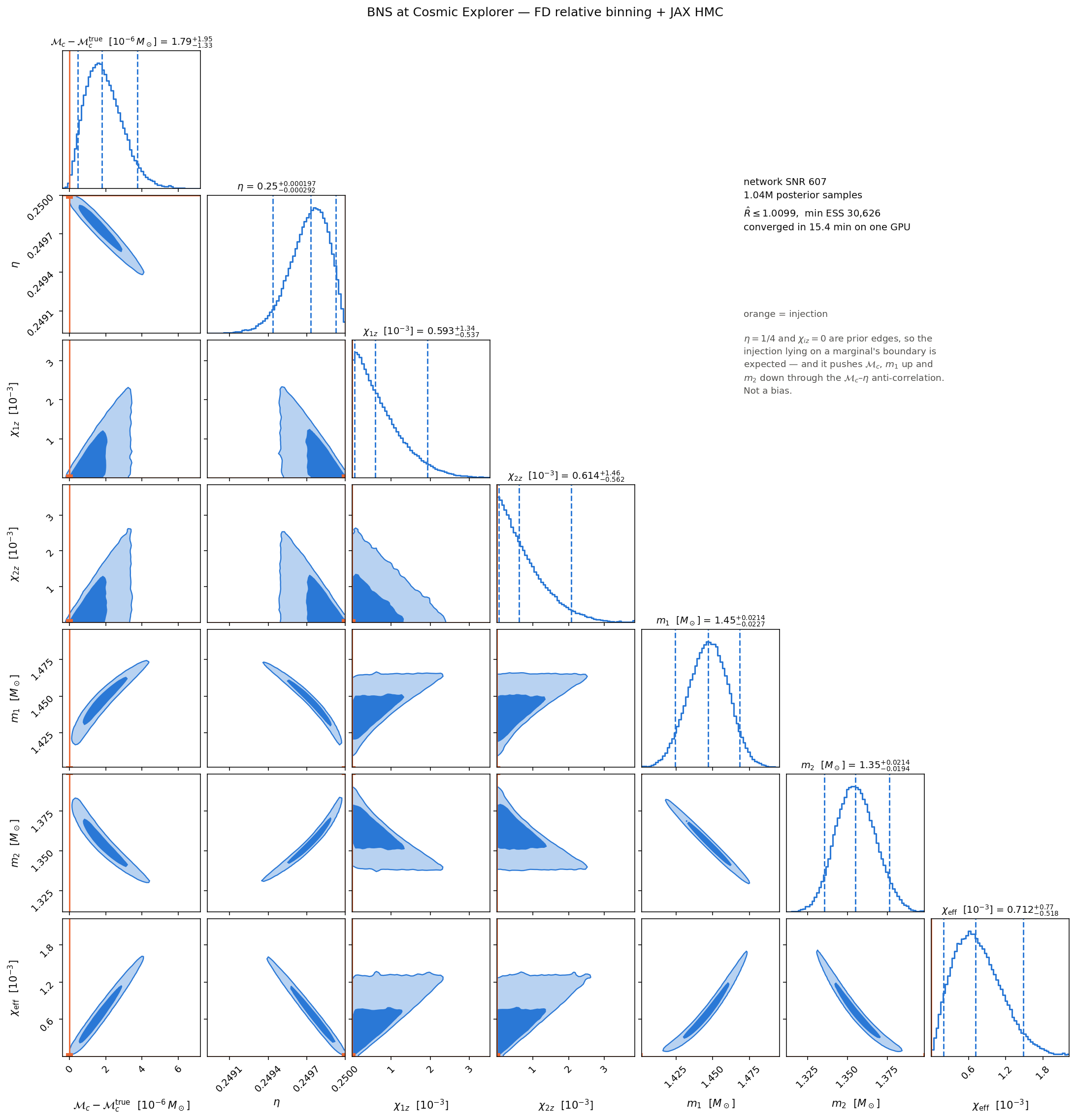
Median chirp mass 1.2187730 M☉ against an injected 1.2187707 — a measurement to roughly one part in 10⁶, which is what SNR 607 over a ~1000 s inspiral buys. Chirp mass is drawn as an offset from the injection because its posterior is only ~10⁻⁶ M☉ wide. The three right/bottom-most panels — m1, m2, χ_eff — are not themselves sampled; they are computed per-sample from (chirp_mass, η, spin1z, spin2z), the same map used everywhere else on this page, so they can be read off directly instead of reconstructed by hand from the sampled corner.

The marginals are one-sided about the truth by construction, not biased. Truth recovery comes out at +1.84 σ in chirp mass, −1.86 σ in η and ~+1 σ in both spins, and those same offsets appear in the 15.4-minute reference. The injection sits exactly on the η = 0.25 prior boundary; Mc and η are ~97 % anti-correlated, so truncating η from above truncates Mc from below (and, equivalently, pushes m1 up and m2 down — visible directly in their panels now). The spin panels show the expected χ_eff degeneracy triangle — only the mass-weighted combination is measured, so the individual spins slide along the anti-diagonal until the positive-support priors cut them off, which pushes their medians above zero and η’s below its truth; the χ_eff panel makes that combination explicit — it is the actual spin quantity this measurement constrains, not the individual spins.

Nothing is tuned to this source

A standing constraint on this work: no per-binary tuning, and no changes to the physics of the templates — no dropping waveform content, no reduced-frequency-content approximations, no reduced precision in template evaluation. Every timing on this page evaluates the full three-region IMRPhenomD in float64. All the speedups are sampler-side; in particular the flow supplies Metropolis–Hastings proposals, so the target density is preserved exactly however good or bad the flow happens to be.

Component masses are --mass1/--mass2, η’s truth follows from them, priors and the optimiser start are derived at runtime, and every adaptation is driven by measured acceptance. Verified by rerunning a 1.35 + 1.25 M☉ injection with no retuning: it converges (R̂ 1.0097, chirp mass recovered exactly, same boundary signature), picks its own step sizes, and passes relative-binning parity on its own waveform.

The configuration carries over; the wall clock does not. That source needs 41 blocks and ~5.0 min rather than 25 and 3.5 min — it is simply a harder posterior, and it needed proportionally more blocks under every earlier configuration too. Its η truth sits just inside the prior edge (0.24963) rather than exactly on it, trading a pinned corner for a genuinely curved two-dimensional ridge.

One related defect, found and fixed: --max-production-blocks defaulted to 40, which the unequal-mass run hit at R̂ = 1.0107 and therefore reported as not converged. It needed 42. A cap that turns “needs slightly longer” into “failed” is measuring the cap; --max-minutes is the real budget guard, and the default is now 80.

Beyond BNS: a mass sweep to 80 M☉

The 1.35 + 1.25 M☉ check above verifies the configuration survives a slightly unequal BNS. bin/run_mass_sweep_pe.py pushes the same question much further: six equal-mass injections, log-spaced in total mass from 2.8 M☉ (BNS) to 80 M☉ (BBH), each run unmodified through this page’s exact HMC + flow pipeline via run_bns_ce_pe.py — same code, same defaults, only --mass1/--mass2, segment duration, and distance change per injection. Duration is sized per injection from LALSimulation’s own chirp/merger/ringdown time bounds rather than reusing 2048 s everywhere (a 40+40 M☉ signal is in band for ~5 s from 10 Hz); distance is solved to a comparable-but-not-identical network SNR (~18–23) via the exact 1/D scaling now exposed as --target-snr on run_bns_ce_pe.py itself.

M_tot (M☉)	SNR	duration	bins	blocks	s/block	time to converge	R̂_max	min ESS
2.80 (BNS)	21.6	2048 s	125	28	3.66	3.39 min	1.0098	9,492
5.47	19.6	512 s	125	32	3.68	3.33 min	1.0097	12,617
10.70	22.2	256 s	125	20	3.66	2.60 min	1.0092	12,185
20.93	21.2	64 s	125	12	3.76	2.10 min	1.0099	9,741
40.92	17.6	32 s	125	9	4.06	1.88 min	1.0074	10,833
80.00 (BBH)	22.9	8 s	124	8	3.97	1.80 min	1.0096	14,623

Bin and block counts are read from each injection’s run.log; unlike the stage timings they are not in the committed CSV.

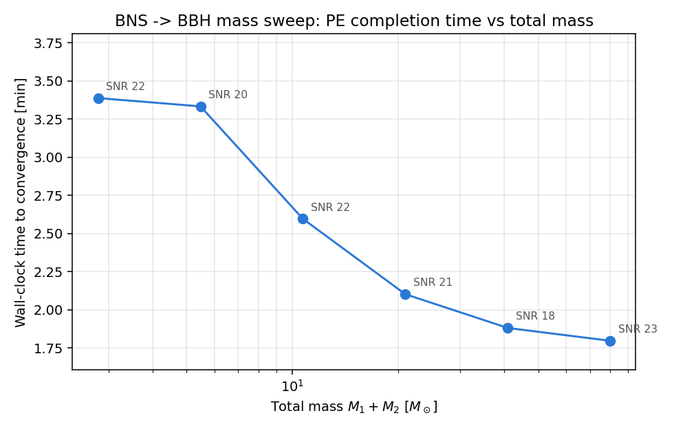
All six converge on the same R̂/ESS gate as everywhere else on this page, and completion time falls monotonically with mass, 3.39 → 1.80 min, rather than growing or non-monotonically wandering. That direction was an assumption in the “What is left” section below until this sweep measured it.

The mechanism is not the one originally claimed here. The obvious reading — higher mass, shorter segment, fewer relative-binning bins, therefore cheaper per gradient — is wrong on both halves, and the sweep’s own artefacts say so. Bin count is set by --epsilon, not by mass: the logs record 3754394 band points -> 125 bins at 2.8 M☉ and 14666 -> 124 bins at 80 M☉, with every injection in between also at 125. Cost per gradient is flat too — warmup is a fixed 5 blocks, so its wall clock probes that cost directly, and it varies by 2 % (13.76–14.03 s) across a 29× mass range. Per production block is flat to 11 % and, if anything, rises with mass.

What falls is the block count to convergence, 28 → 8. This is a mixing result, not a cost result. The remainder of the decline is the CPU-side setup that genuinely does scale with segment duration (injection, SNR rescale, RB summary, RB validation: 29.0 s at 2.8 M☉ → 12.2 s at 80 M☉), sitting on a ~38 s floor (MAP+Laplace, warmup, flow fit) that does not move at all. Why mixing improves with mass is not established here — the natural reading is that fewer in-band cycles leave a broader, less curved M_c–η ridge, but this sweep measures the block count, not the mechanism behind it.

None of this is proof the sampler’s hyperparameters (flow spline interval, equilibration rounds, …) are optimal all the way to 80 M☉, only that the BNS-tuned defaults, left untouched, still reach the same convergence gate there.

Raw sweep output: mass_sweep_summary.csv; figure via python bin/plot_mass_sweep_timing.py <sweep_summary.csv>.

Posteriors across the sweep

Same layout as the BNS corner plot above — chirp mass, η, spin1z, spin2z, plus the derived m1, m2, χ_eff (χ_eff = (m1·spin1z + m2·spin2z)/(m1+m2)) panels appended, truth marked throughout — one per injection, in increasing total mass. The table below is the same derived quantities made quantitative (median and 90% CI), for reference without opening every image:

M_tot (M☉)	m1 truth / median [90% CI]	m2 truth / median [90% CI]	χ_eff truth / median [90% CI]
2.80	1.400 / 1.650 [1.526, 1.760]	1.400 / 1.194 [1.125, 1.286]	0 / 0.017 [0.005, 0.032]
5.47	2.737 / 3.278 [3.016, 3.500]	2.737 / 2.300 [2.166, 2.489]	0 / 0.023 [0.007, 0.040]
10.70	5.352 / 6.393 [5.886, 6.779]	5.352 / 4.508 [4.272, 4.875]	0 / 0.024 [0.007, 0.041]
20.93	10.464 / 12.444 [11.427, 13.189]	10.464 / 8.853 [8.391, 9.598]	0 / 0.025 [0.008, 0.042]
40.92	20.458 / 24.188 [22.281, 25.726]	20.458 / 17.411 [16.436, 18.835]	0 / 0.025 [0.009, 0.042]
80.00	40.000 / 46.705 [42.930, 49.955]	40.000 / 34.484 [32.293, 37.452]	0 / 0.025 [0.009, 0.041]

m1/m2 are one-sided about the truth for the same reason chirp-mass/η are (see above): η is truncated at its true value of exactly 0.25, so the posterior only ever sees eta <= eta_true, which pushes m1 up and m2 down at every mass — this is a prior boundary artifact, not a mass asymmetry the sampler invented. χ_eff is similarly one-sided because the spin priors are (Uniform(0, 0.05) on each of spin1z/spin2z, not centered on 0), so a mass-weighted average of two positive-truncated quantities comes out positive even when both truths are exactly 0. Both effects are visible directly in the corner plots below and are already discussed for the BNS case earlier on this page; the table above is the same statement made quantitative at every mass in the sweep.

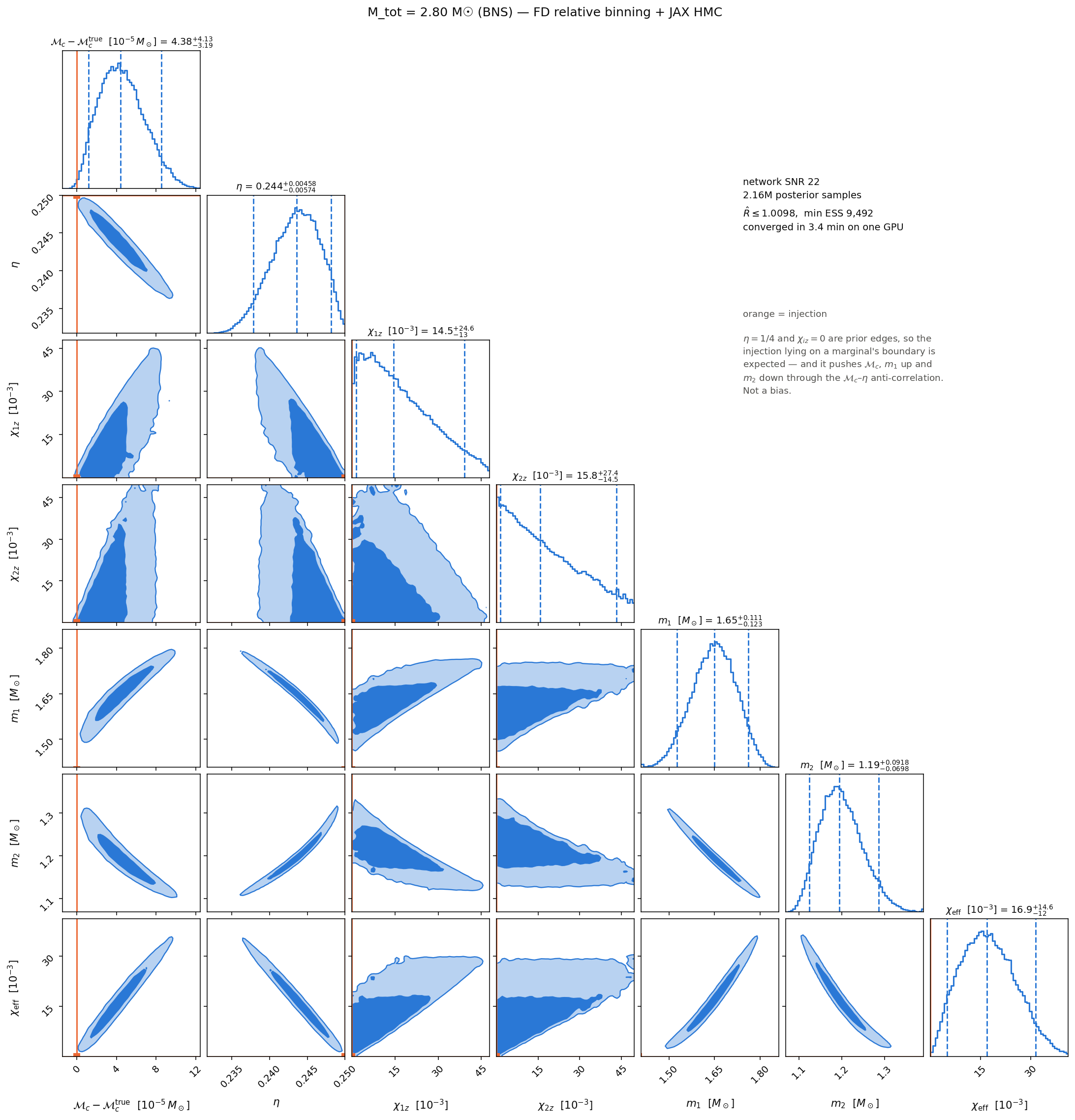
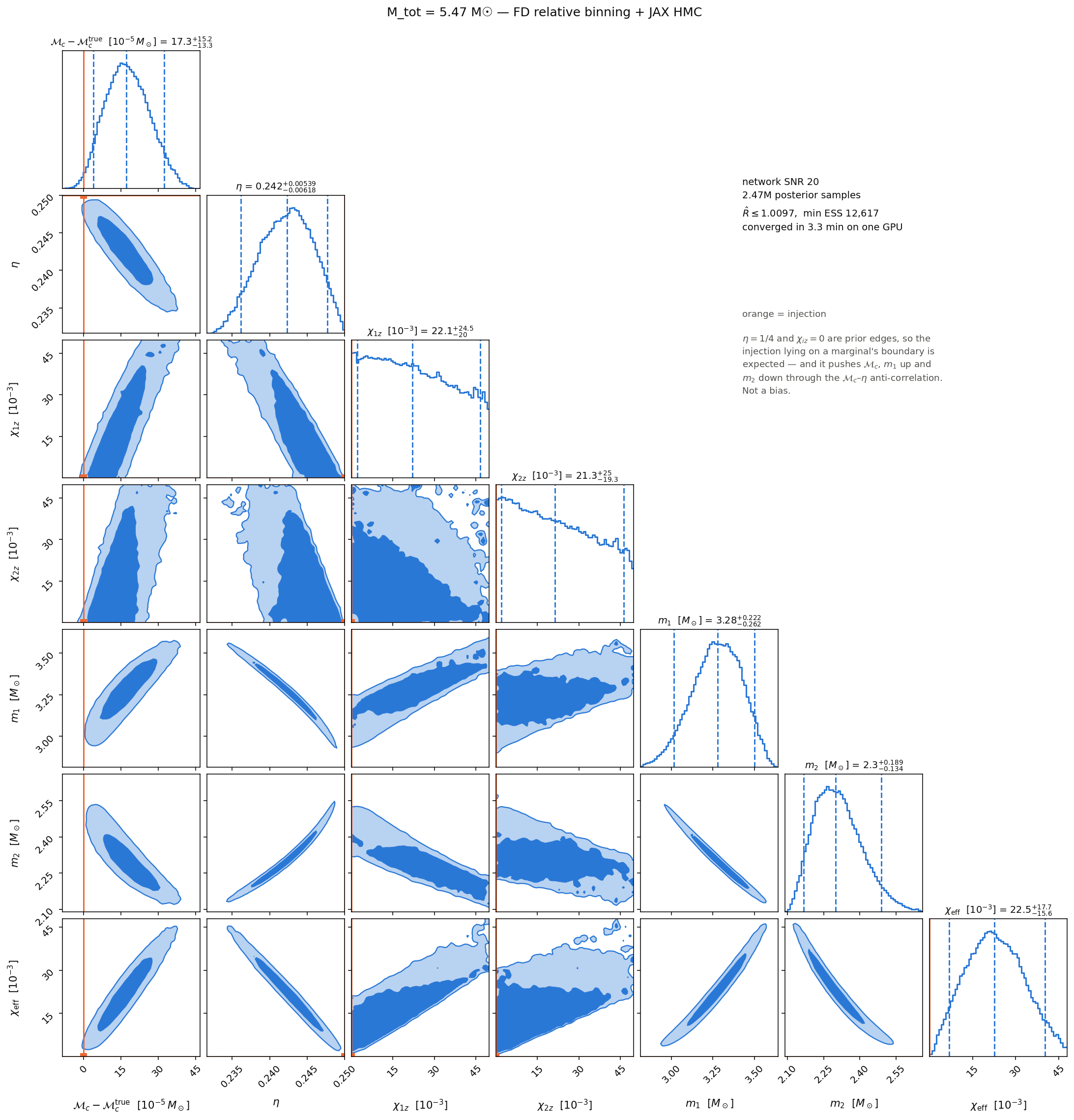
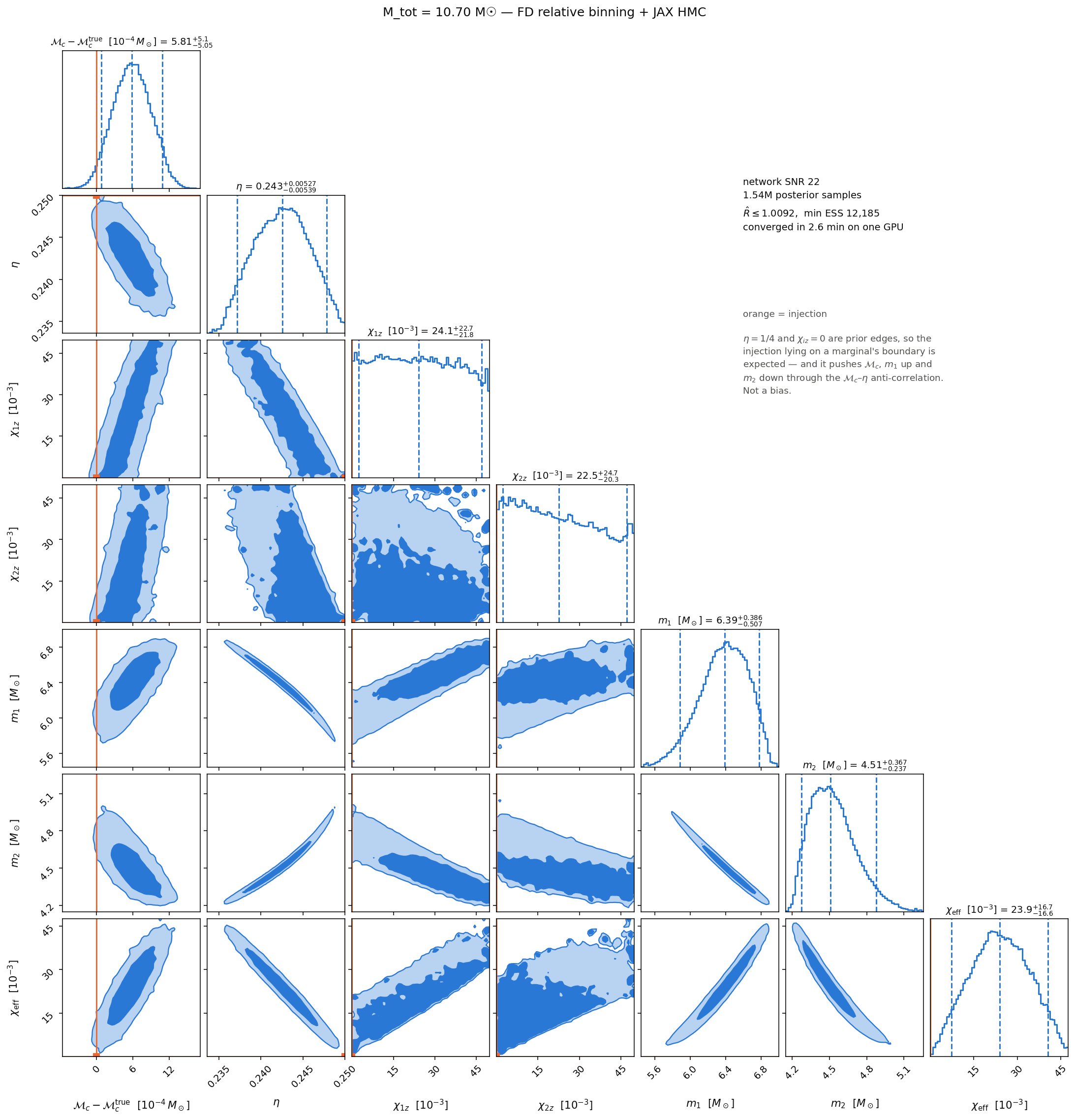
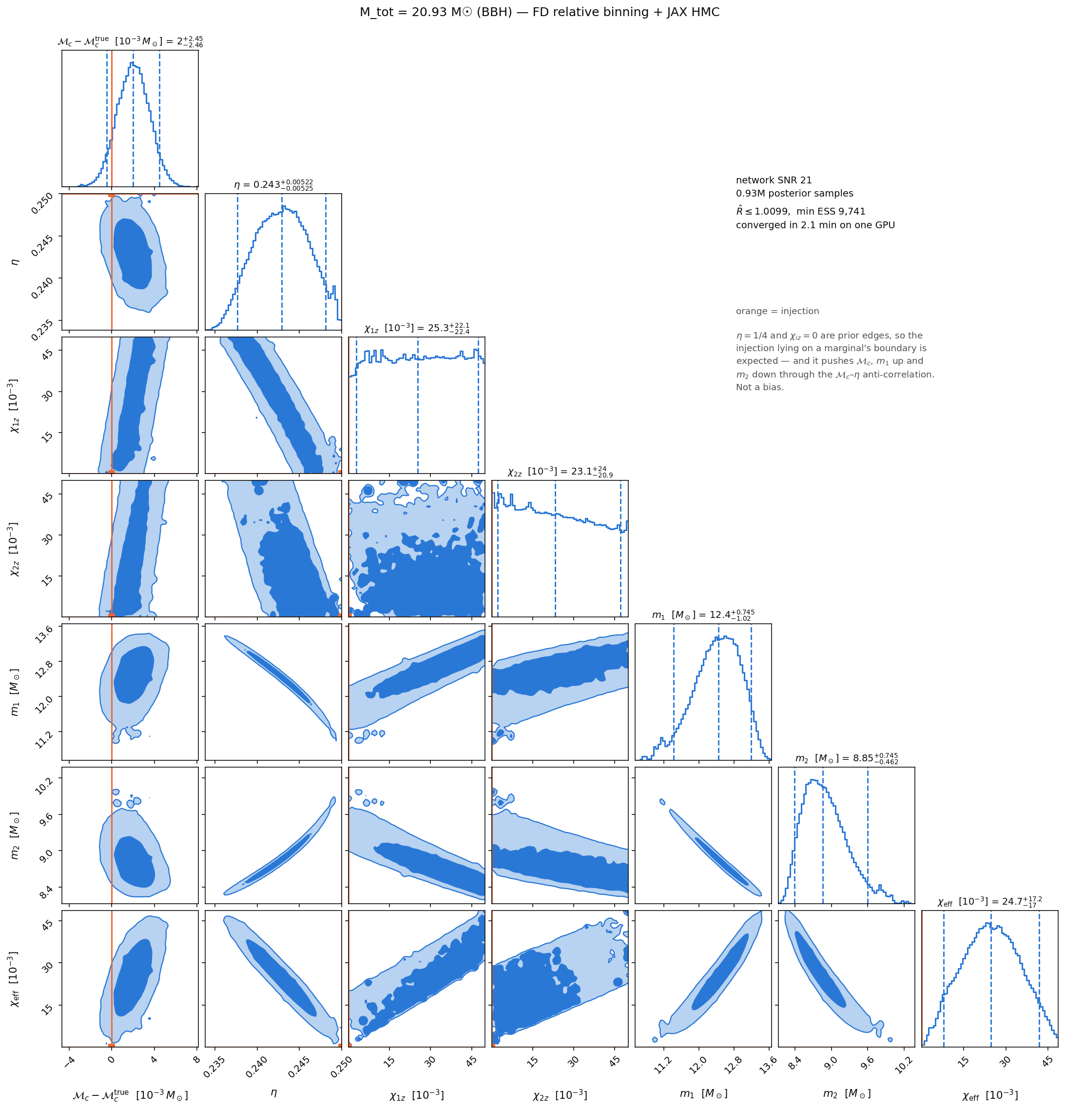
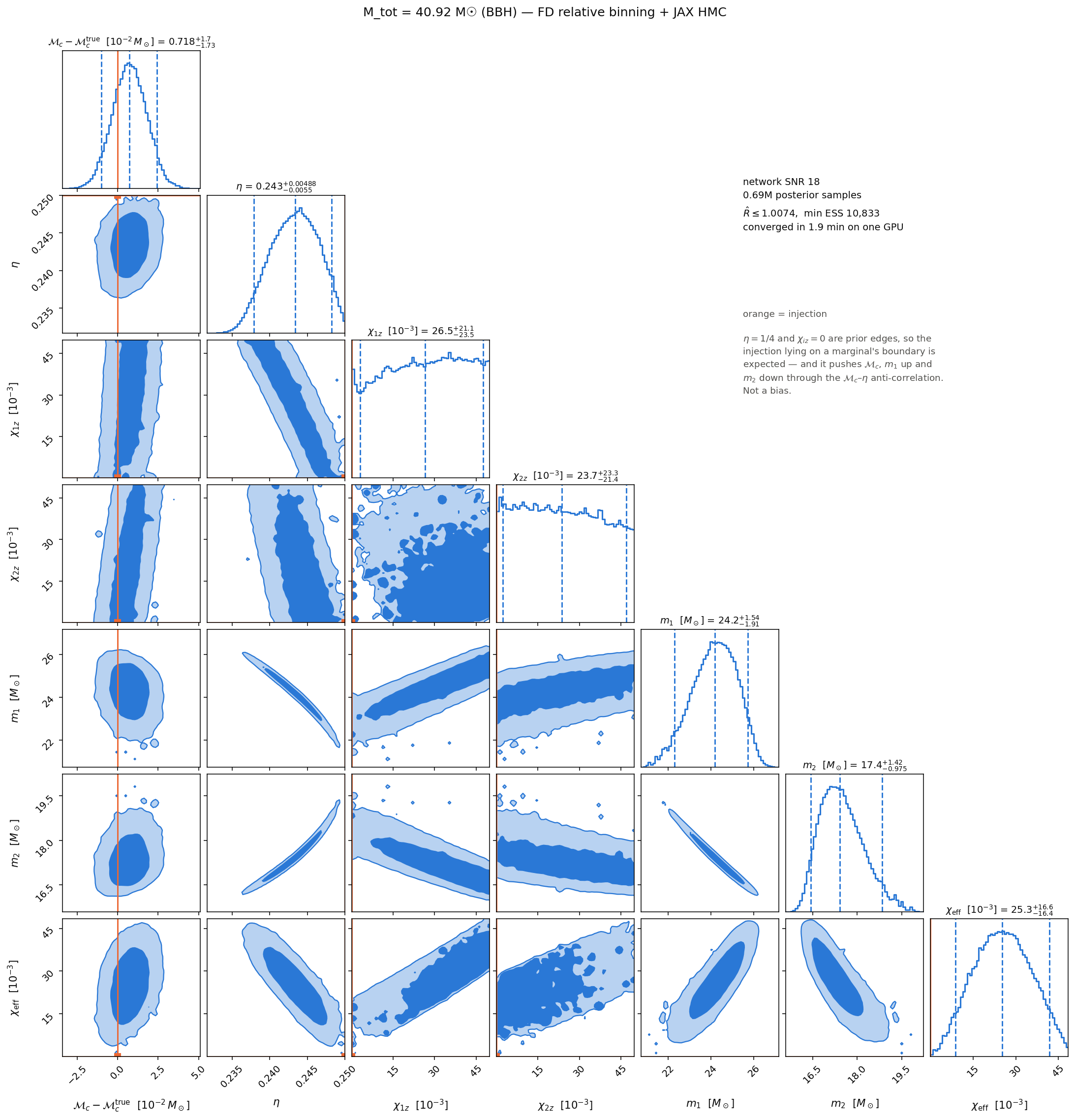
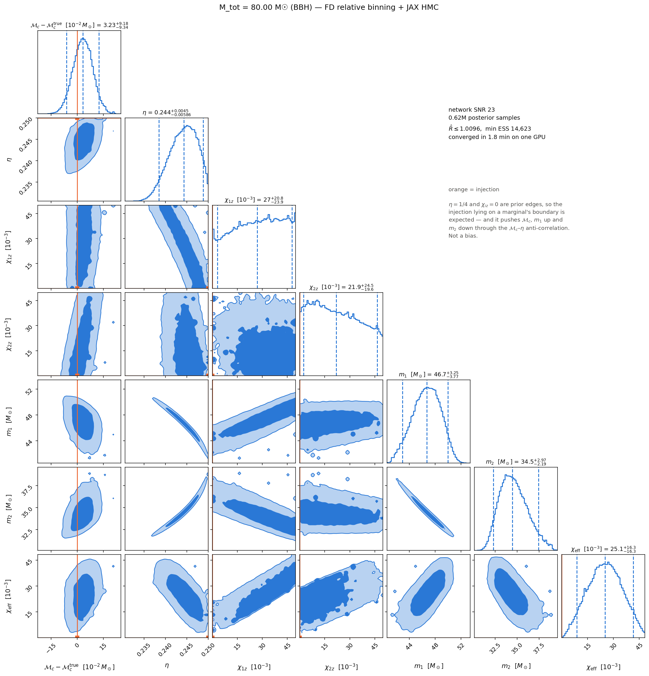
A trend is visible across the set that has nothing to do with sampler performance and everything to do with the physics: the spin1z/spin2z marginals flatten as mass increases. At 2.8 M☉ they peak sharply at zero and fall off by z ~ 0.03; by 10.7 M☉ they are already close to flat; by 80 M☉ they are indistinguishable from the uniform [0, 0.05] prior. A higher-mass signal spends fewer inspiral cycles in band before merger, and it is the accumulated spin-orbit phasing over many cycles that measures spin — fewer cycles means less of that signature, independent of how well the sampler mixes. The chirp-mass/η anti-correlation (the same one described for the BNS case above) persists at every mass, since it comes from the η = 0.25 prior boundary, not from the source.

These six runs predate the MAP start-point fix described in the next section. They used a fixed 2 % inset off the prior edge; the optimiser start is now chosen from a ladder. At these masses with a narrow zero-centred spin prior the difference is immaterial — but the numbers above were measured before it, and have not been re-run.

---

Spinning binaries, and all five transition kernels

Everything above holds spins near zero: the reference BNS injects χ₁ᶻ = χ₂ᶻ = 0 under a one-sided Uniform(0, 0.05) prior. That turns out to be a load-bearing assumption in two places that have nothing to do with the sampler, and both surface immediately when the suite is pushed to realistic aligned spins.

The suite: ten equal-mass injections, log-spaced from 2.8 to 80 M☉, each component classified NS below 3 M☉ and BH at or above, aligned-spin truth drawn per component from ±0.05 (NS) or ±0.9 (BH), recovery prior widened to the symmetric range of the wider component, distance solved per injection to a comparable-but-not-identical network SNR (~18–23). Each is then sampled by all five jaxpe.kernels transition kernels on the same 90-minute budget and the same R̂ < 1.01 / ESS ≥ 2000 gate used everywhere else here. Seven of the ten are reported: the other three refine to 6 375–7 900 relative-binning bins and are measured below as infeasible on this hardware.

Two defects a ±0.9 spin prior exposed

1. The MAP optimiser started in the wrong place, and failed silently. The Laplace mass matrix comes from a damped-Newton MAP started at the fiducial point, inset off any prior edge it lies on (the sigmoid bijection sends open bounds to ±∞, so a start exactly on a boundary is not representable). That inset was a fixed 2 % of the prior width. Because the injection is zero-noise, lnL peaks at exactly 0 at the fiducial, so the inset’s cost is directly measurable — and at 55 M☉, insetting η by 0.02 × 0.05 = 10⁻³ costs 392 nats. Newton then starts 392 below the peak, climbs monotonically exactly as designed, and still terminates at a prior corner (η = 0.2, χ₁ᶻ = χ₂ᶻ = −0.9) whose Laplace covariance has σ ~ 10⁻¹³. Nothing raises; the run proceeds to sample with a mass matrix that is numerically a delta function.

The optimiser is now run from every rung of a ladder (2×10⁻² … 2×10⁻⁶) and the best converged mode is kept, rejecting any whose Laplace covariance has collapsed. Selecting on the rung’s starting log-posterior — the obvious cheaper version — is wrong, and measurably so: for the zero-spin BNS that criterion picks the 2×10⁻⁴ rung, which climbs to a mode pinned against the η boundary at log-posterior −26.8 with a smallest σ_y of 6.8×10⁻⁷, where the 2×10⁻² rung reaches −17.6 at 4.3×10⁻⁶, a metric 6× wider in its tightest direction. Newton only accepts improvements, so every rung is a valid local ascent; which basin it lands in is what the start decides, and only the final mode reveals that.

Re-running the reference BNS confirms the validated path is unchanged: the ladder keeps 2×10⁻² (log-posterior −17.6, against −20.0 / −26.8 / −33.5 / −40.4 for the finer rungs), converges at R̂ = 1.0098 with min ESS 21 846, and recovers chirp mass 1.21877 against an injected 1.21877.

Caveat on the suite below. The best-converged-mode criterion was found while performing that reference check, after the ten-injection suite had already been run against a shared setup cache built with the cheaper start-log-posterior criterion. Rebuilding the cache both ways and comparing: the two criteria select different rungs on most injections, but converge to essentially the same mode anyway — the resulting Laplace covariances agree to within 3 % on eight of ten. The exceptions are 26.2 M☉ (1.77× wider in its tightest direction under the corrected criterion) and 38.0 M☉ (57×, one of the three that never produced a result). So the caveat is narrow but not empty, and it is not neutral for the cross-kernel comparison: a metric that is too tight penalises single-step kernels far more than HMC.

The suite below has since been re-run in full against the corrected cache, so the results reported here are no longer subject to this caveat. It is kept because the difference mattered: measured against the corrected metric, the cross-kernel divergences that the first pass reported (12–32× the Monte-Carlo floor) fall to 3.6–5.1×. A metric defect that agrees to 3 % on eight of ten injections still moved the headline conclusion of a kernel comparison by roughly a factor of four.

2. Relative-binning resolution is set by the prior volume, not the source. The heterodyne’s linear-in-f ratio model must hold across the parameters actually proposed, so widening the spin prior from ±0.05 to ±0.9 at SNR ≈ 20 breaks it: measured RB-vs-dense tail ratios of 0.22–0.50 against a 5×10⁻³ tolerance, 40–100× outside contract. --epsilon now auto-refines (quartering, tolerances never relaxed) until the existing parity guard passes. The cost is real and is recorded per injection: half the grid needs 490–7 900 bins where the BNS reference needs 125.

Neither is visible at BNS masses with narrow spin priors, which is why both survived.

Making it a fair comparison

The solved distance, refined --epsilon, and MAP+Laplace mode and covariance depend only on the injection, never on the kernel. They are derived once per injection and shared across all five sweeps via --setup-cache, so every kernel samples a bit-identical likelihood from a bit-identical mass matrix and any difference is a difference between kernels alone. Two further corrections were needed before the comparison meant anything:

• --max-production-blocks was binding instead of the time budget. At its previous default of 80, MALA hit the cap on 6 of 10 injections having spent only 6.4 of its 12 allowed minutes. A fixed block cap penalises exactly the kernels that take smaller steps per block, so the comparison would have measured the cap. Default raised to 400.
• The 12-minute budget itself was binding, and it was the single largest source of “did not converge” in the first pass of this suite: 13 of 35 runs ended on production wall-clock budget exhausted with R̂ still falling monotonically block over block and no stuck chains. Those were unfinished runs, not failures. Raised to 90 minutes, which converts every one of them except MMALA’s two. A budget-limited run is reported as not converged either way — the point is that reading it as a statement about the kernel was wrong.
• ULD’s step size was never a measured choice. It has no acceptance signal to adapt on, so --step-size is held fixed for the whole run, and the first pass left it at the default of 0.5 while the MH kernels’ own adaptation selected 0.006–0.033 on these same posteriors. Running an unadjusted integrator at 15–80× the step the geometry supports does not measure the cost of dropping the accept/reject step; it measures a broken step size. It now takes MALA’s adapted value per injection via --step-size-from, and the difference is not subtle — see the ULD discussion below.

• Everything runs on CPU, not the GPU — because mid-suite the CUDA driver wedged (cuInit → CUDA_ERROR_UNKNOWN, while nvidia-smi continued to report a perfectly healthy card). This is a fallback, not a preference: measured per production block, the T2000 is 1.9–2.6× faster than this CPU (see “Different hardware” below). What matters for the comparison is only that all five kernels ran on the same device; absolute wall clocks here are therefore ~2.3× the GPU figures quoted elsewhere on this page and should not be compared across sections.

  A caution worth recording, since it nearly went into this page as a result: an early CPU-vs-GPU comparison appeared to show the CPU winning, because the GPU side of it was measured while the driver was already degrading (per-block cost had silently tripled before it failed outright). The healthy-GPU numbers say the opposite. run_mass_sweep_pe.py --require-gpu now creates and exercises a real CUDA context before the first injection and aborts if it cannot; nvidia-smi is documented there as explicitly not a valid readiness check.

Results

30 of 35 runs pass the gate. End-to-end minutes on identical CPU hardware, against the corrected setup cache and the 90-minute budget:

M_tot (M☉)	bins	HMC	MALA	MMALA	RandomWalk	ULD
2.8	125	✅ 21.8	✅ 19.1	✅ 19.7	✅ 12.5	✅ 20.9
4.1	499	✅ 69.0	✅ 69.0	✗ R̂ 1.0136	✅ 42.8	✅ 50.1
5.9	125	✅ 11.4	✅ 17.1	✅ 17.8	✅ 10.1	✅ 10.7
8.6	499	✅ 64.8	✅ 46.8	✗ R̂ 1.0320	✅ 60.7	✗ R̂ 1.0355
26.2	125	✅ 26.1	✗ R̂ 1.0129	✅ 35.4	✅ 48.6	✅ 61.9
55.1	490	✅ 46.5	✅ 62.4	✅ 35.5	✅ 35.7	✅ 35.6
80.0	124	✅ 13.1	✅ 31.0	✅ 42.1	✅ 31.4	✗ R̂ 1.0114

✅ = passed the gate, with end-to-end minutes; ✗ = budget exhausted, with the R̂ reached. HMC and RandomWalk are 7/7, MALA 6/7, MMALA and ULD 5/7. The earlier reading of this table — that bin count, not kernel, decides whether a run converges — was an artefact of too small a budget: with 90 minutes the 490+ bin injections converge for almost everything, and the two remaining MMALA failures are the longest runs in the suite (96 and 95 minutes) rather than the most expensive posteriors.

Passing the gate and getting the right answer are not the same thing, and this suite separates them in both directions. ULD at 55.1 M☉ converged — R̂ 1.0095, ESS 7531 — and is 51× the Monte-Carlo floor away from HMC on η. MALA at 26.2 M☉ and ULD at 80.0 M☉ failed the gate and are statistically indistinguishable from HMC (0.9–2.6× and 0.5–2.0× the floor). R̂ measures whether chains agree with each other, which is not the same as agreeing with the target; the next subsection measures the second thing.

Three injections are absent from this table entirely (12.4, 18.0 and 38.0 M☉, the ones the parity guard pushed to 6 375–7 888 bins), and they are the clearest statement of what the refinement costs. Re-run alone with a 25-minute budget, the 12.4 M☉ case spends 617 s in warmup, 950 s in equilibration, and then 325 s per production block, reaching only R̂ = 1.13 after four blocks. Extrapolating the block count these posteriors need, each run is hours, and the fifteen runs (three injections × five kernels) are tens of hours on this hardware. They were abandoned rather than reported as fast failures; no sampler was given an advantage, because none of them got a result.

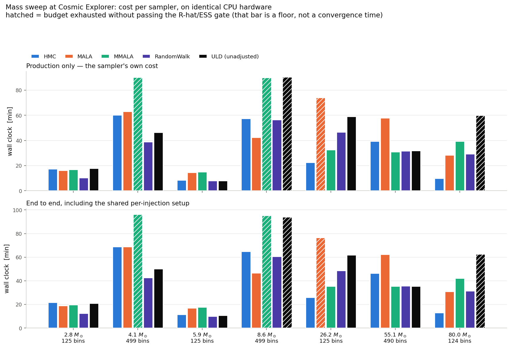
The figure is grouped by binary rather than plotted against mass on purpose. Along that axis mass co-varies with two quantities the six-injection sweep above held fixed, and both move cost more than mass does.

Bin count, through the ε refinement. Warmup is a fixed 5 blocks, so its wall clock probes per-gradient cost directly: 53–84 s at 125 bins against 149–178 s at ~490 bins — 2.26× the cost for 4.0× the bins (≈ bins^0.59, not the near-flat scaling that holds at 125 bins on the GPU). The abandoned 12.4 M☉ case is a third point on the same curve and lands on the same exponent: 617 s of warmup at 6 375 bins is 8.7× the 125-bin cost for 51× the bins, or bins^0.55. The three 490+ bin runs are exactly the three most expensive HMC runs; separation by bin count is perfect. And because the refinement is a hard-threshold quartering ladder, it is discontinuous in mass rather than trending with it: 4.1 M☉ needs 499 bins under narrow NS spin priors, while 26.2 and 80.0 M☉ need 125 under ±0.9.

Spin prior width, through the NS/BH classification at 3 M☉ per component. The chirp-mass prior is ±10 % of truth and η is always [0.2, 0.25], so spin is the only prior box that differs from the sweep: (0, 0.05) there against ±0.05 or ±0.9 here — 18× wider per dimension, stepping partway along the mass axis at M_tot ≈ 6 M☉.

Control for both and HMC’s mass scaling is the same as the sweep’s. Every homogeneous subgroup declines:

subgroup	end-to-end minutes, in increasing mass
125 bins, ±0.05 spin	2.8 → 21.8, 5.9 → 11.4
125 bins, ±0.9 spin	26.2 → 26.1, 80.0 → 13.1
~490 bins	4.1 → 69.0, 8.6 → 64.8, 55.1 → 46.5

The last row is not prior-homogeneous — 4.1 M☉ is ±0.05, the other two ±0.9 — so it mixes both effects; the first two rows are clean. The offset between those two rows is the prior-width cost made visible: at a common 125 bins, 26.2 M☉ costs more than 2.8 M☉, inverting the sweep’s ordering entirely, which puts the ±0.9 penalty at roughly 3× (a displacement from the within-tier trend, not a fit). So the non-monotonicity here is produced by interleaving three cost tiers along one axis, and a line against a mass axis would draw neither the trend that exists nor the one it appears to show.

Two limits on this decomposition: the per-kernel run logs are not retained, so it rests on the stage timings in the committed CSVs with no production block counts to check it against; and these runs shared a 12-core CPU two at a time, the likely source of the 53–84 s scatter within the 125-bin warmups where the GPU sweep’s equivalent scatter is 2 %.

Medians agree; the distributions differ at the boundary

Posterior medians against HMC’s, in units of HMC’s own posterior σ, worst over all four sampled parameters and all seven binaries:

kernel	worst median shift vs HMC
MALA	0.48 σ (η, 8.6 M☉)
MMALA	0.40 σ (η, 8.6 M☉)
RandomWalk	0.17 σ (η, 8.6 M☉)
ULD	0.50 σ (η, 55.1 M☉)

All four land in the right place to within half a σ. A median is one number from a four-dimensional distribution, and it is the number every kernel here gets right.

Jensen–Shannon divergence against HMC (same estimator as compare_bns_posteriors.py) is more discriminating. Referred to a null built by splitting HMC’s own chains in half — the honest Monte-Carlo floor, since any two finite samples of the same distribution have JS > 0 — the median over all 28 (binary, parameter) pairs is:

kernel	median	worst
RandomWalk	1.7× floor	6.7× (η, 55.1 M☉)
ULD	3.5×	51× (η, 55.1 M☉)
MALA	3.6×	26× (η, 8.6 M☉)
MMALA	5.1×	37× (η, 55.1 M☉)

This is the number that most changed when the suite was re-run properly. The first pass of this comparison put MALA and MMALA at 12–32× the floor and concluded the MH-corrected kernels were substantially under-dispersed relative to HMC. Against the corrected mass matrix and an adequate budget the medians are 3.6× and 5.1×. Most of that gap was a suboptimal shared metric being amplified by single-step kernels, not a property of the kernels — which the earlier text could only spot-check on one binary and now holds across all seven.

What survives is narrower, one-sided, and concentrated at the prior boundary. Every non-HMC kernel returns a narrower 90 % credible interval than HMC on almost every parameter of every binary: median width ratios 0.80 (MALA), 0.84 (MMALA and ULD), 0.92 (RandomWalk), and only 0–11 % of the 28 comparisons come out wider at all.

The sharpest discriminator is the η = 0.25 pileup — the feature this page’s sampler was built around (“the η → 1/4 and spin → 0 pileups that no fixed mass matrix equilibrates”). Fraction of the posterior within 10⁻³ of that edge:

M_tot (M☉)	HMC	MALA	MMALA	RandomWalk	ULD
2.8	15.9 %	0.11 %	5.3 %	9.6 %	1.5 %
8.6	3.4 %	0.00 %	0.22 %	1.2 %	0.00 %
26.2	9.0 %	3.1 %	3.7 %	6.5 %	5.9 %
55.1	13.9 %	1.8 %	0.37 %	5.5 %	0.01 %
80.0	14.4 %	7.6 %	10.5 %	10.6 %	8.8 %

HMC reaches the boundary more than every other kernel on every binary, and the ordering (HMC, then RandomWalk, then MMALA/MALA/ULD) is the same ordering as the JS table. The 55.1 M☉ row is the extreme case and is visible directly in that binary’s corner figure: because η = 0.25 means m₁ = m₂, a kernel that misses the pileup pushes the derived m₁ marginal to higher masses, and ULD’s modal m₁ sits at 35.0 M☉ against HMC’s 29.2 (the injected value being 27.6).

Is HMC right, or merely different? Two arguments that it is the least truncated, and one reason to keep the question open. η_true = 0.25 exactly for these equal-mass injections and is a hard prior edge, so genuine posterior mass there is expected, and HMC’s η median is the closest to truth on every binary checked. The unconstrained-space bijection sends η = 0.25 to +∞, so reaching it requires long excursions, and HMC’s 32 leapfrog steps travel ~32× further per proposal than any single-step kernel — the mechanism predicts exactly the observed ordering. But this is an argument from mechanism plus a self-consistency check, not an independent verification of the boundary mass; nothing here measures it against a reference that is not itself one of these samplers.

ULD needs its previous entry on this page retracted. The first pass reported it as catastrophically broken: up to 27 % non-finite draws, JS 0.15–1.00 against a ~0.005 floor, a chirp-mass median 218 σ from HMC’s, and never passing the gate at any mass. Every one of those numbers was measuring a step size of 0.5 that nothing had chosen — 15–80× what the MH kernels’ adaptation selects on the same posteriors. Run at MALA’s adapted step per injection, ULD produces zero non-finite draws, a worst median shift of 0.50 σ, a median JS of 3.5× the floor, and passes the gate on 5 of 7 binaries. It is an ordinary member of this comparison, not an outlier.

The genuine cost of dropping the accept/reject step is narrower and better localised: ULD has no Metropolis correction, so its stationary distribution carries an O(ε²) discretisation bias by construction (jaxpe/kernels/uld.py) and does not converge to the right answer at any run length at fixed ε. That bias is what the 55.1 M☉ result shows — converged by R̂ (1.0095, ESS 7531), 51× the floor from HMC on η, and 0.01 % boundary occupancy against HMC’s 13.9 %, i.e. 1400× less. Its chains agree with each other and disagree with the target. This is the honest measurement of the unadjusted tradeoff, and it is much smaller than the previous text claimed while being a sharper statement of the same thing.

Two structural caveats that no amount of budget addresses: mala, uld and random-walk use their scale elementwise in jaxpe.kernels, so they receive per-dimension marginal standard deviations rather than the dense Cholesky factor hmc and mmala get, and cannot see the ~97 % M_c–η anti-correlation at all; and mmala runs in its documented constant-metric mode, which its own docstring calls equivalent to dense-mass MALA, not the full Riemannian variant. Only hmc has tuned numbers behind it here — the others use jaxpe’s library-default acceptance targets, which are literature values not measured on this posterior, and production acceptance drifts well off even those. Retuning them is a confound this suite does not remove.

Posteriors, all samplers overlaid

One figure per binary, every kernel on common axes, injection marked. The 1-D marginals are densities rather than counts — the kernels return different numbers of samples, and a count histogram would read a longer run as a taller posterior. Axis ranges are the union of each kernel’s 0.5–99.5 percentile box, so a kernel that sampled somewhere else widens the frame rather than vanishing off the edge of its own comparison.

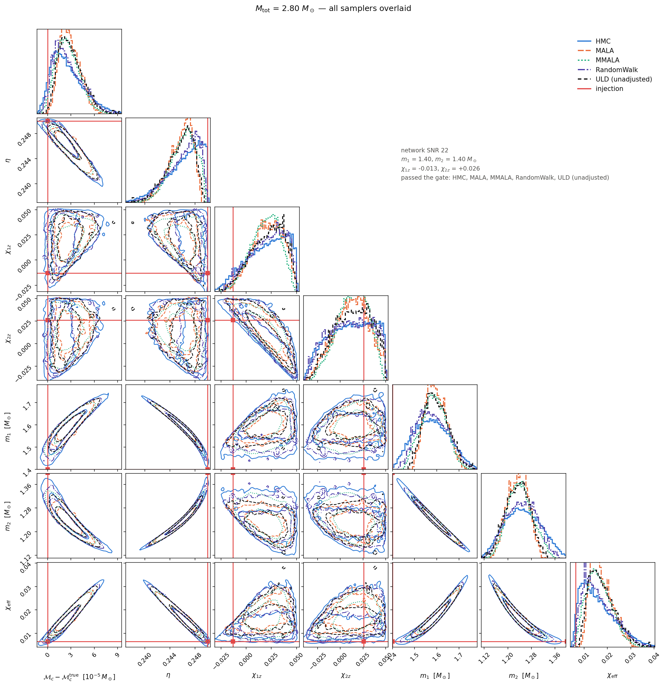
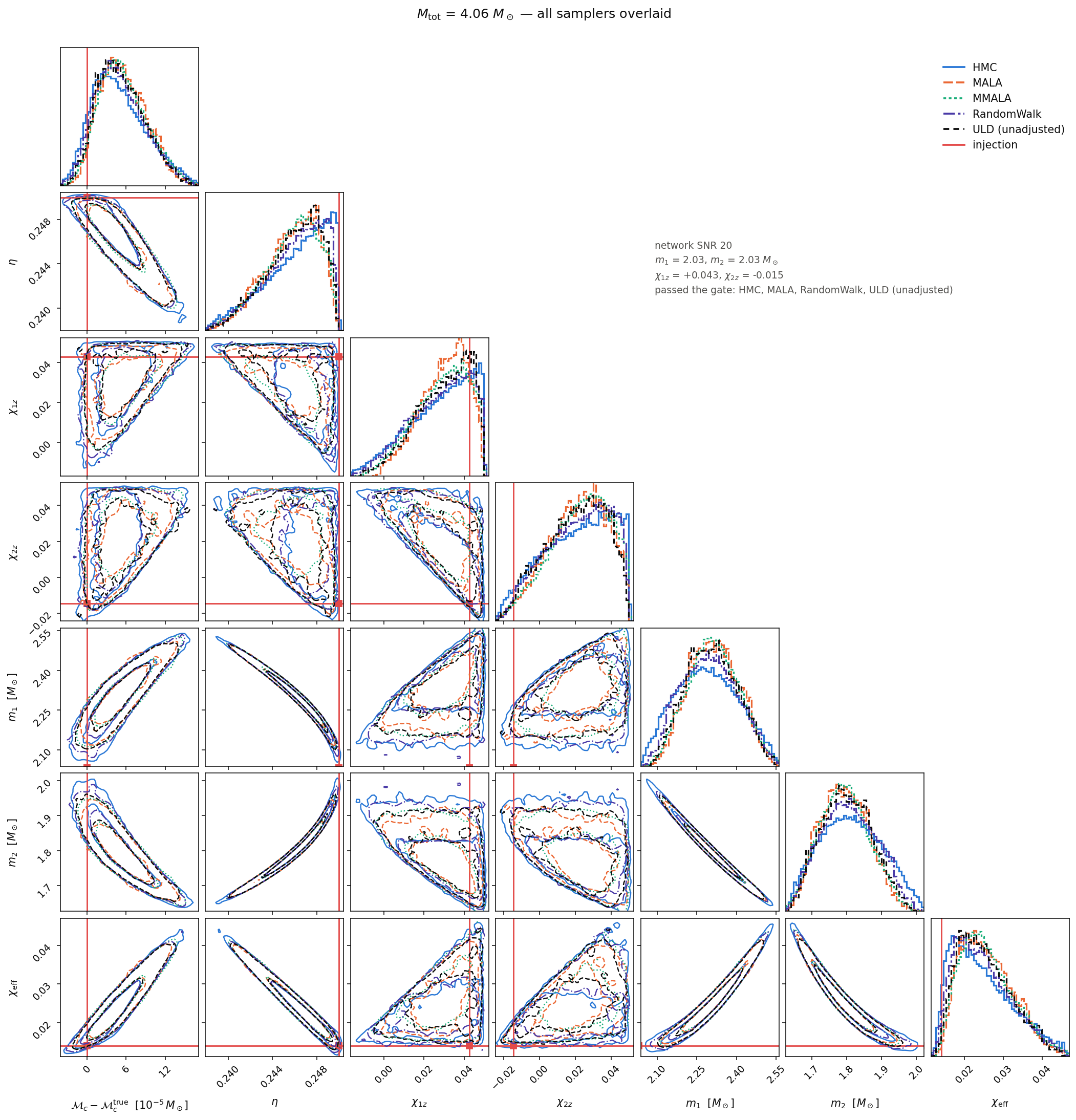
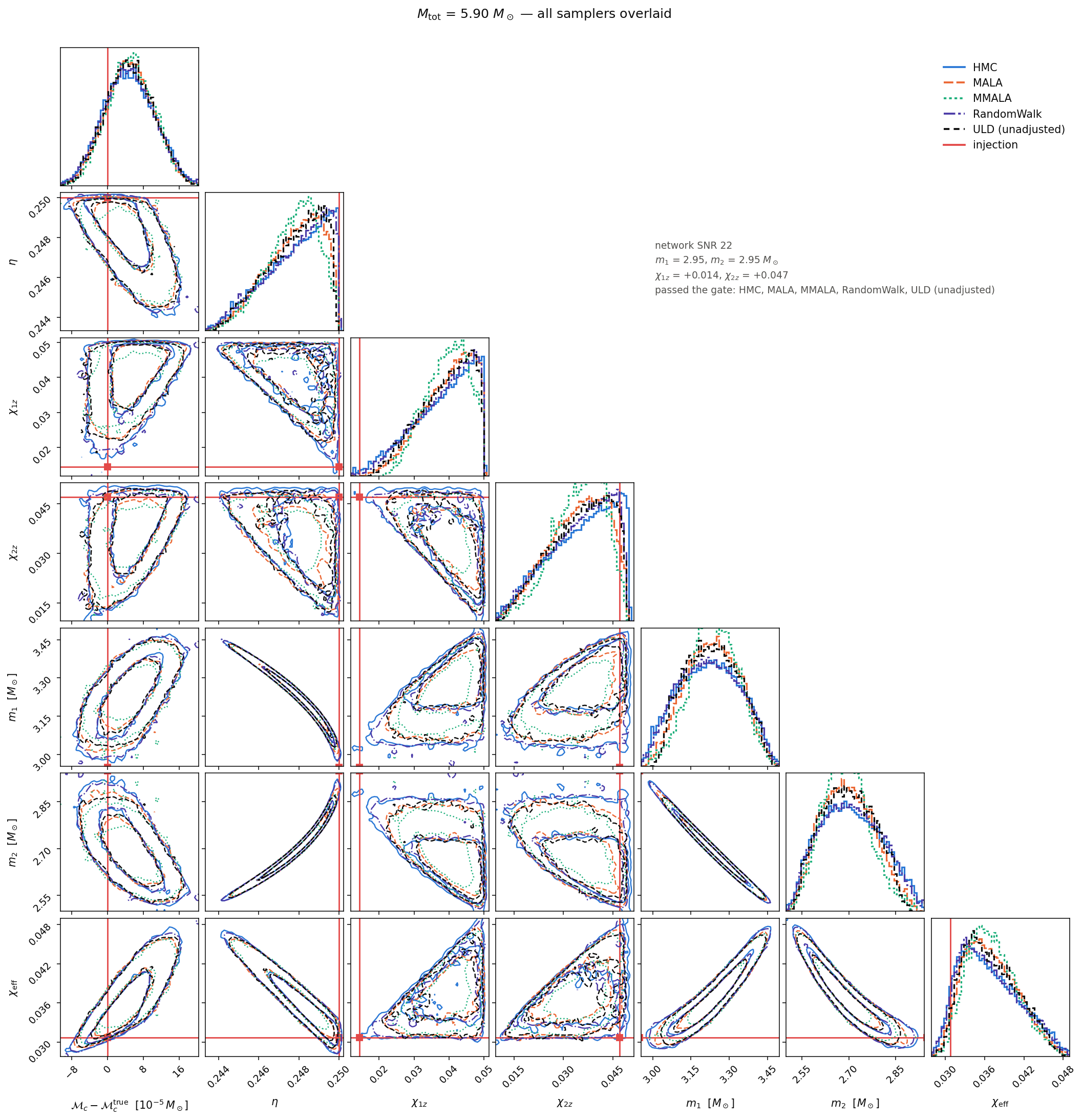
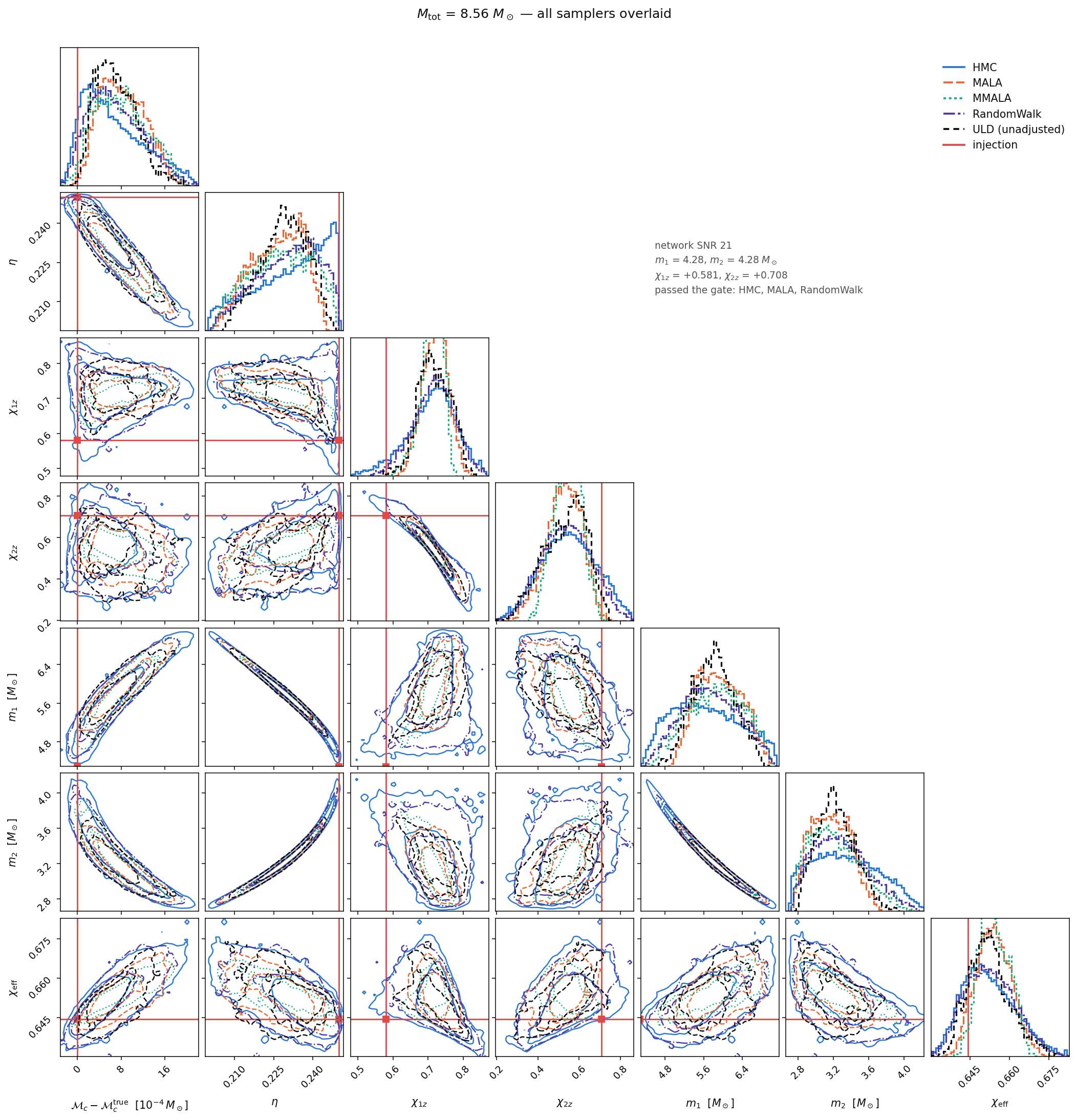
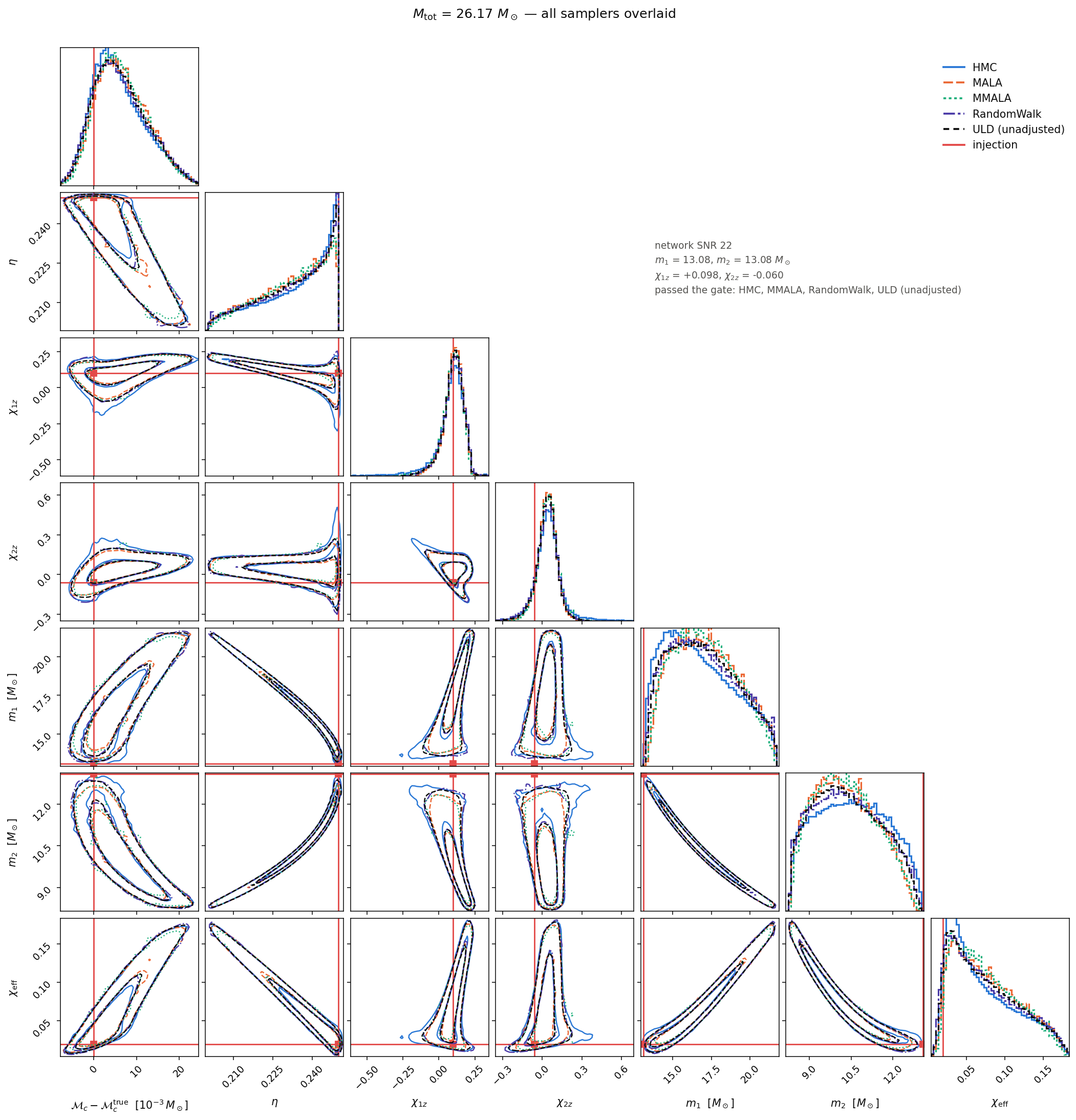
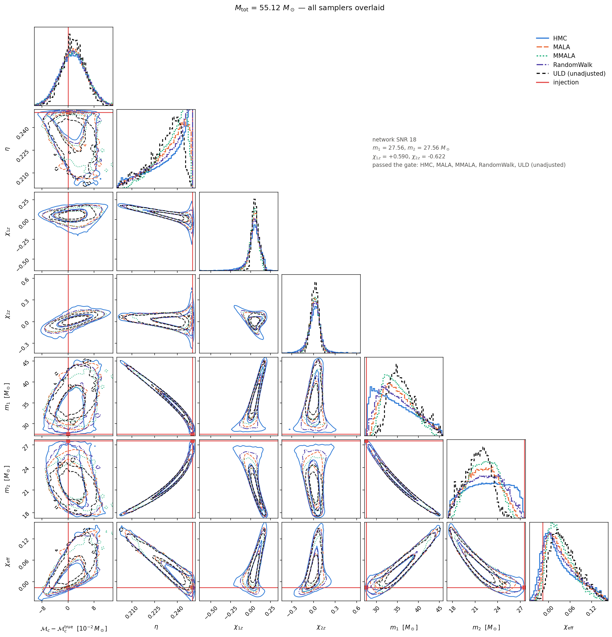
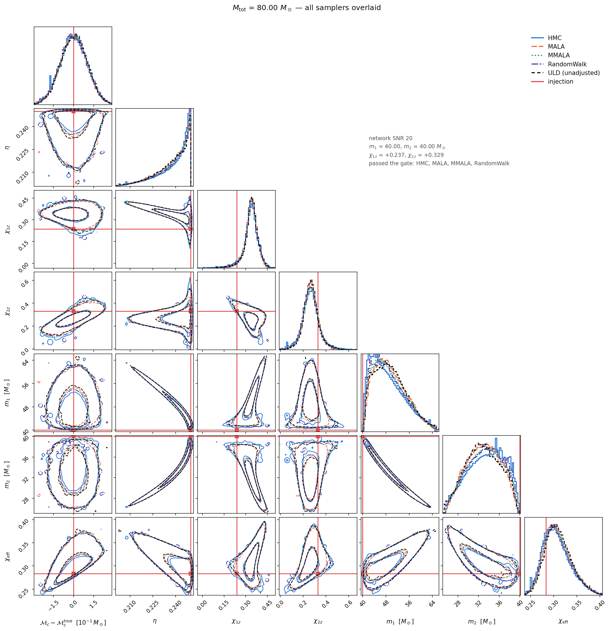
All five contour sets now sit on top of one another in most panels of most figures — including ULD’s, which in the first pass of this suite sat somewhere else entirely. Where they separate, they separate at the η = 0.25 edge and in the m₁/m₂ marginals that edge controls. The 55.1 M☉ figure is the one to read: every kernel passed the gate there (the info box lists all five), yet ULD’s m₁ marginal peaks at 35.0 M☉ where HMC’s peaks at 29.2 against an injected 27.6 — entirely because ULD put 0.01 % of its samples against the equal-mass boundary and HMC put 13.9 %. A figure in which every curve overlaps and one derived marginal does not is the clearest picture on this page of what the convergence gate does and does not certify.

The spin panels show the expected χ_eff physics at these SNRs: individual aligned spins are barely measured, and at 55.1 M☉ the injected +0.590/−0.622 pair (χ_eff ≈ −0.016) recovers as two broad marginals peaked near zero with the combination constrained — which is why χ_eff is carried as its own panel rather than left to be reconstructed.

Raw per-kernel output: sampler_sweep_hmc.csv and the four alongside it. Figures via python bin/make_sampler_comparison_figures.py --root <sweep root>.

---

What is left, if you want to go further

Production is still ~55 % of the run, and the dominant term is the IMRPhenomD gradient itself: a long serial dependency chain (~3600 instructions, 5 fusions) whose cost is sublinear in chains and — at this benchmark’s 125 bins on the T2000 — nearly flat in bin count. That flatness is a small-n, latency-bound regime rather than a general property: on CPU the same gradient costs 2.3× more at ~490 bins and 8.7× more at 6 375 bins, i.e. roughly bins^0.55–0.6 (see the five-kernel section). Trajectory length is at its measured knee, the flow is at its measured knee, and both halves of the preamble are load-bearing in both directions.

• Different hardware. fp64 throughput is what matters here, and it is not a professional-versus-consumer distinction: the T2000 and the A40 both run fp64 at 1/32 of fp32. A100/H100-class parts (1/2 rate) are the ones that change this arithmetic. A larger card also lifts the 4 GB constraint that forces setup onto the CPU, and makes large chain counts cheap enough to be worth revisiting.

  The CPU is closer than the fp64 rates suggest, but does not win. Measured per production block on four injections, the T2000 is 1.9–2.6× faster than the 12-core Xeon W-10855M (4.1–5.3 s/block against 10.1–10.4 s/block). That is a far smaller margin than a GPU-versus-CPU comparison normally implies — the card’s 1/32 fp64 rate puts it near 40 GFLOPS against ~149 GFLOPS fp64 measured on the CPU, and the GPU wins anyway on memory bandwidth and on vmapping 64 chains — but it does mean a CPU-only run of this pipeline is perfectly practical, at roughly 2.3× the wall clock.

• A cheaper exact gradient, e.g. a reduced-order or surrogate waveform. That is a different accuracy contract from trimming PhenomD and needs its own validation.
• Skipping unused waveform regions is ruled out, not deferred. Phase/Amp evaluate all three frequency regions and select with heaviside masks, and JAX evaluates both sides of a where. Timed end to end, eliminating the unused ones caps out at ~6 % of the run — the 4× HLO instruction-count ratio badly overstates it, because those instructions are cheap elementwise work over 126 points. Not worth editing a 4000-line waveform module for, and it falls under the template constraint regardless.

---

Reproducing the figures

python bin/make_bns_ce_figures.py     # reads examples/output/bns_ce_rb_hmc/
python bin/make_sampler_comparison_figures.py --root <dir of per-kernel sweeps>

The five-kernel sweep behind that second figure, on a machine with two GPUs. The setup cache must be built once and serially first — it is what makes every kernel sample a bit-identical likelihood and mass matrix, and two concurrent sweeps pointed at an empty cache dir race to write the same file:

ROOT=examples/output/sampler_sweep
COMMON="--n-injections 10 --max-minutes 90 --setup-cache $ROOT/cache --require-gpu"

CUDA_VISIBLE_DEVICES=0 python bin/run_mass_sweep_pe.py $COMMON \
    --outdir $ROOT/_setup --extra-args --setup-only

CUDA_VISIBLE_DEVICES=0 bash -c 'for k in hmc mmala; do
    python bin/run_mass_sweep_pe.py '"$COMMON"' --kernel $k --outdir '"$ROOT"'/$k; done' &
CUDA_VISIBLE_DEVICES=1 bash -c 'for k in mala random-walk; do
    python bin/run_mass_sweep_pe.py '"$COMMON"' --kernel $k --outdir '"$ROOT"'/$k; done' &
wait

# uld last: it has no acceptance signal to adapt on, so it takes MALA's adapted
# step size per injection rather than a default nothing chose
CUDA_VISIBLE_DEVICES=0 python bin/run_mass_sweep_pe.py $COMMON \
    --kernel uld --outdir $ROOT/uld --step-size-from $ROOT/mala

bin/make_bns_ce_figures.py rebuilds all three figures from run artefacts, so every number on the axes traces back to a measurement rather than to this page. The convergence series and the per-configuration stage timings are cached to bns_ce_convergence.csv and bns_ce_speed_stages.csv — raw run logs fall under the repository’s *.log ignore, so those CSVs are the committed evidence and the figures regenerate from a clean checkout. The corner plot needs samples.npz (~1–2M × 4 float64, deliberately untracked); rerun the PE to regenerate it.

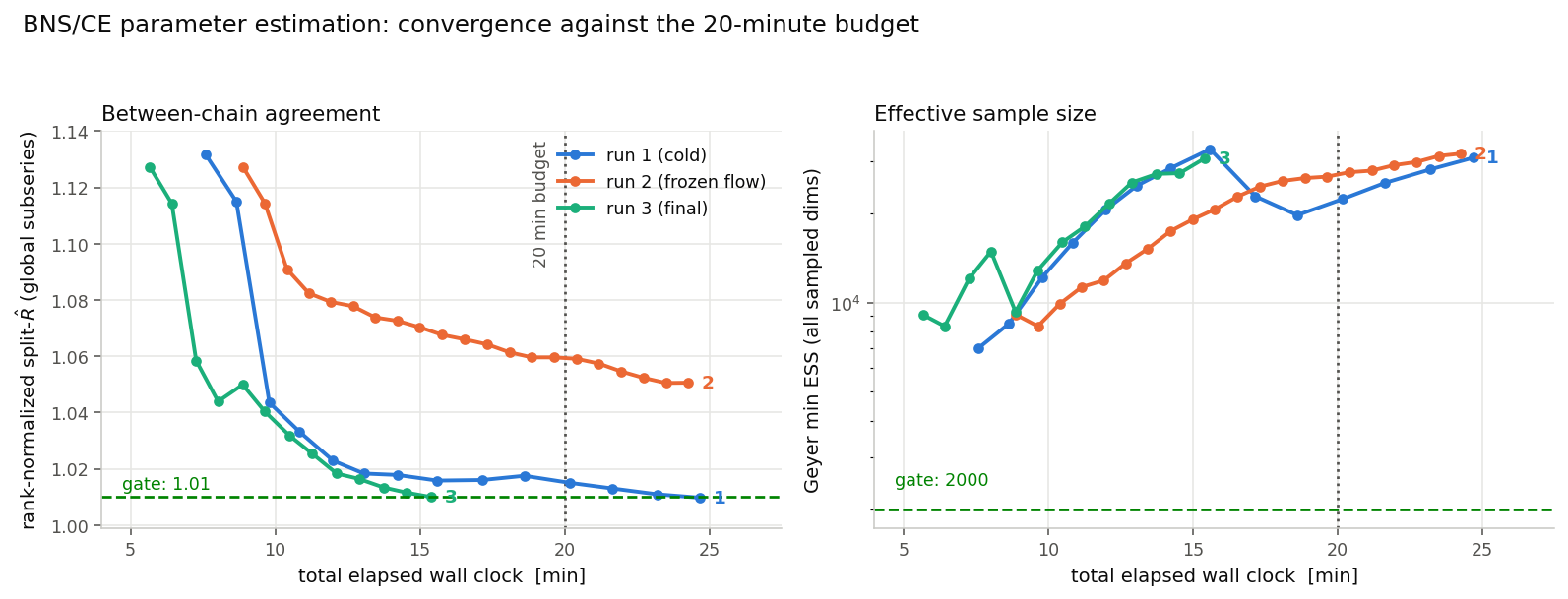
This figure is from the original 20-minute-budget round and is kept for the failure mode it captures: the run that froze its flow (middle series) kept accumulating ESS at a healthy rate while R̂ plateaued near 1.05 and never converged. That divergence between ESS and R̂ is the signature of a proposal that produces samples but does not move chains between the boundary tails.

Notes

• The maximum sampled log-posterior (−15.48) exceeds the damped-Newton “MAP” (−18.14). There is no sharp finite mode: the boundary directions are flat until the sigmoid Jacobian turns over, so Newton stops early on a plateau. This affects only where the preconditioner is centred, and production acceptance of 0.7–0.8 says the metric is fine.
• Diagnostics use the global subseries for R̂ because plain split-R̂ over the raw autocorrelated series asymptotes at √(1 + 4τ/n) — it re-measures within-chain autocorrelation and would need ~400τ samples to certify 1.01. The raw value is reported alongside for reference.
• Profile on the backend you actually run on. Diagnostics timed under JAX_PLATFORMS=cpu do not bound the same code on the GPU, and a standalone vmap(grad(loglike)) differs measurably from the same gradient inside a scan over an HMC trajectory (3.2 vs 4.5 ms here) — the standalone figure is the one that misled.