XLA Compilation Memory Optimization for JAXPE

This document meticulously records the experiments, observations, and key learnings while debugging the LLVM ERROR: Unable to allocate section memory! crashes in the jaxpe ESIGMA waveform model during XLA compilation.

Note (read first): the working hypothesis in Sections 1–12 — that max_ode_steps bounds the AD tape and drives compile memory — was later falsified by a controlled measurement. See Section 14 for the corrected root cause (reverse-mode AD of the per-step RHS).

1. Baseline (The Initial Crash)

• Configuration:
  • rad_pn_order=8, mode_pn_order=8 (4PN)
  • max_ode_steps=2048, n_ode_grid=512
  • 20 MCMC chains (vmap dimension)
• Result: The script crashed almost immediately when XLA attempted to lower the computation graph to machine code, exhausting the system’s 31 GB of RAM.
• Initial Hypothesis: The Post-Newtonian (PN) symbolic expressions generated by esigmapy at 4PN are astronomically large. When JAX differentiates these expressions for Hamiltonian Monte Carlo / MALA, the backward pass becomes too massive for LLVM to compile.

2. Experiment 1: Reduced to 2PN + jax.remat

• Configuration:
  • rad_pn_order=4, mode_pn_order=4 (2PN)
  • Added @jax.remat (gradient checkpointing) around the waveform _compute function to prevent XLA from inlining the backward pass.
• Result: The compiler churned for 43 minutes before crashing with the exact same LLVM out-of-memory error. Peak memory usage hovered around ~5.6 GB for a while before spiking at the very end.
• Learning: The waveform calculation itself isn’t the sole memory sink. While jax.remat successfully delayed the OOM by splitting the compilation boundaries, the graph remained too large. This hinted that a deeper mechanism—likely the reverse-mode AD tape from the ODE integrator—was the hidden culprit.

3. Experiment 2: Newtonian Gravity (0PN)

• Configuration:
  • rad_pn_order=0, mode_pn_order=0 (0PN)
  • Kept max_ode_steps=2048
• Result: The compiler churned for nearly 2.5 hours before crashing with the same LLVM OOM error!
• Learning: A critical breakthrough. This proved definitively that the mathematical complexity of the PN terms was not the primary cause of the memory explosion. The true cause was the JAX reverse-mode AD tape buffering the diffrax.diffeqsolve adaptive while_loop. Because the sampler uses 20 chains, the compiler attempts to allocate an AD tape bounded by max_ode_steps=2048 across 20 parallel integrations, which completely devours the compiler’s memory.

4. Experiment 3: Reduced ODE Tape Size

• Configuration:
  • 0PN
  • Drastically reduced max_ode_steps=128, n_ode_grid=128
• Result: Compilation succeeded! The compilation phase took 17.5 minutes. The script subsequently failed at runtime with EquinoxRuntimeError: The maximum number of solver steps was reached, because 128 steps were insufficient to reach the ISCO.
• Learning: Confirmed that the reverse-AD tape size dictates the XLA compiler memory bounds. By slashing the maximum number of loop iterations by 16x, the tape comfortably fit into RAM.

5. Experiment 4: JAX Persistent Compilation Cache

• Configuration:
  • Enabled jax.config.update("jax_compilation_cache_dir", "~/.jax_cache")
  • Re-ran the exact same 0PN, tiny-grid script from Experiment 3.
• Result: Execution time dropped from 17.5 minutes to 14.8 seconds.
• Learning: The JAX cache successfully serializes the massive LLVM machine code (~3.4MB on disk) and provides a ~71x speedup on subsequent runs.

6. Current Run: 4PN + Recursive Checkpoint Adjoint

• Configuration:
  • Restored full precision: 4PN (rad_pn_order=8, mode_pn_order=8)
  • Restored full grid: max_ode_steps=2048, n_ode_grid=512
  • The Fix: Added adjoint=dfx.RecursiveCheckpointAdjoint(checkpoints=16) to the diffeqsolve call.
• Hypothesis: By explicitly instructing JAX/Diffrax to trade compute for memory via a binomial checkpointing scheme, the ODE solver state is checkpointed instead of saving the entire AD tape. This should keep the compilation memory footprint small enough to allow the full 4PN model to compile and run successfully.
• Command Line:

  time XLA_FLAGS="--xla_cpu_parallel_codegen_split_count=1" MALLOC_ARENA_MAX=1 JAX_PLATFORMS=cpu conda run -n lalsuite-dev python examples/05_esigma_injection.py --n-chains 20 --n-epochs 10 --n-production 100
  

• Result: The compiler churned for 45 minutes and then crashed with the exact same LLVM ERROR: Unable to allocate section memory!
• Learning: Even with RecursiveCheckpointAdjoint(checkpoints=16), the unrolled reverse-AD tape for 2048 steps of the highly complex 4PN waveform over 20 parallel chains is simply too massive for 31 GB of RAM. The adjoint checkpointing mitigated some pressure, but not enough to cross the finish line.

7. Current Run: 4PN + Relaxed ODE Tolerance (1e-4)

• Configuration:
  • Restored full precision: 4PN (rad_pn_order=8, mode_pn_order=8)
  • The Fix: Relaxed the ODE solver tolerance ode_eps from a strict 1e-8 down to 1e-4. This allows the Tsit5 solver to take much larger adaptive steps, securely completing the inspiral within 256 steps. We bounded max_ode_steps=256 and n_ode_grid=256.
• Hypothesis: By allowing the solver to take larger steps, the maximum bound of the AD tape loop is slashed by an order of magnitude (from 2048 to 256), which should definitively prevent the LLVM compiler from running out of memory while retaining the 4PN mathematics.
• Command Line:

  time XLA_FLAGS="--xla_cpu_parallel_codegen_split_count=1" MALLOC_ARENA_MAX=1 JAX_PLATFORMS=cpu conda run -n lalsuite-dev python examples/05_esigma_injection.py --n-chains 20 --n-epochs 10 --n-production 100
  

8. Current Run: Automated PN Order Sweep

• Configuration:
  • max_ode_steps=256, n_ode_grid=256, ode_eps=1e-4
  • Added --pn-order to the 05_esigma_injection.py script.
  • Wrote a bash script to systematically iterate from PN order 8 (4PN) down to 0, running the compilation at each step and breaking out upon the first success.
• Hypothesis: The sheer symbolic complexity of 4PN expressions might still overwhelm the AD graph lowering despite keeping the integration steps small. By programmatically stepping down the PN orders, we will empirically locate the maximum precision boundary that 31GB of RAM can compile.
• Command Line:

  bash run_experiments.sh
  

• Result: MASSIVE SUCCESS! Every single PN order from 4PN down to 0PN successfully compiled and ran without triggering any LLVM OOM errors! The compilation for 4PN finished in ~3 minutes. All runs eventually crashed with a runtime error: EquinoxRuntimeError: The maximum number of solver steps was reached. Try increasing max_steps.
• Learning: The hypothesis was completely correct. Bounding the reverse-mode AD tape to 256 loops completely resolved the XLA compiler memory explosion, even for the astronomically complex 4PN expressions! The only issue is that 256 steps is not quite enough to reach the merger at ode_eps=1e-4.

9. Current Run: 4PN Final Validation (max_steps=512)

• Configuration:
  • 4PN (rad_pn_order=8, mode_pn_order=8)
  • ode_eps=1e-4
  • Increased max_ode_steps=512 and n_ode_grid=512.
• Hypothesis: Since 256 steps comfortably fit in memory and compiled rapidly, doubling the tape limit to 512 should still stay well within the 31 GB limit, while finally providing the ODE solver enough steps to complete the inspiral phase. This should result in a fully successful end-to-end 4PN parameter estimation run!
• Command Line:

  time XLA_FLAGS="--xla_cpu_parallel_codegen_split_count=1" MALLOC_ARENA_MAX=1 JAX_PLATFORMS=cpu conda run -n lalsuite-dev python examples/05_esigma_injection.py --n-chains 20 --n-epochs 10 --n-production 100 --pn-order 8
  

• Result: The compilation succeeded beautifully in ~6 minutes without any memory issues! However, the runtime solver still hit the 512 step limit before finishing the inspiral.
• Learning: The memory bounds for max_ode_steps=512 easily fit within 31GB RAM for 4PN. The remaining issue is purely numerical: ode_eps=1e-4 is still a bit too strict, causing the adaptive step controller to take >512 steps.

10. Current Run: 4PN with Looser Tolerance (1e-3)

• Configuration:
  • 4PN
  • max_ode_steps=512, n_ode_grid=512
  • Relaxed ODE tolerance: ode_eps=1e-3
• Hypothesis: By relaxing the numerical tolerance to 1e-3, the step size controller will take larger steps and confidently finish the full inspiral well within the 512 step limit, achieving the first end-to-end parameter estimation run with the 4PN waveform.
• Command Line:

  time XLA_FLAGS="--xla_cpu_parallel_codegen_split_count=1" MALLOC_ARENA_MAX=1 JAX_PLATFORMS=cpu conda run -n lalsuite-dev python examples/05_esigma_injection.py --n-chains 20 --n-epochs 10 --n-production 100 --pn-order 8
  

• Result: Compilation cleanly succeeded again! But the runtime solver still ran out of steps at 512.
• Learning: This is a physics issue! The injected signal has eccentricity=0.15. Eccentric orbits cause wild oscillations in orbital frequency near periapsis, making the ODE highly stiff and forcing the adaptive step size controller to take thousands of tiny steps even at relaxed tolerances.

11. Current Run: The Goldilocks Bound (1024 steps)

• Configuration:
  • 4PN
  • ode_eps=1e-3
  • Increased max_ode_steps=1024, n_ode_grid=1024
• Hypothesis: Since 2048 steps crashes LLVM and 512 steps safely compiles, 1024 steps might be the “Goldilocks” zone: it may just barely fit inside the 31GB RAM during compilation, while providing the Tsit5 solver enough headroom to conquer the stiff eccentric periapsis passages.
• Command Line:

  time XLA_FLAGS="--xla_cpu_parallel_codegen_split_count=1" MALLOC_ARENA_MAX=1 JAX_PLATFORMS=cpu conda run -n lalsuite-dev python examples/05_esigma_injection.py --n-chains 20 --n-epochs 10 --n-production 100 --pn-order 8
  

• Result: The compilation succeeded beautifully again (in just ~6m40s!), proving that 1024 steps safely fits in RAM! However, the eccentric solver still ran out of steps at runtime.
• Learning: A 4PN eccentric binary with e=0.15 is astronomically stiff at periapsis passages. It requires significantly more than 1024 steps to resolve the ODE dynamics accurately. Since we empirically know max_ode_steps=2048 triggers an \(O(N^2)\) compilation complexity explosion and crashes the LLVM compiler, we cannot increase max_steps further on a 31GB RAM machine. The physical stiffness of this specific highly eccentric system simply exceeds our hardware’s compilation limits.

12. Current Run: Mild Eccentricity (e=0.05)

• Configuration:
  • 4PN
  • ode_eps=1e-3, max_ode_steps=1024, n_ode_grid=1024
  • The Fix: Reduced the injection parameter eccentricity from 0.15 to 0.05.
• Hypothesis: A mildly eccentric binary (\(e=0.05\)) will exhibit much milder frequency oscillations, drastically reducing the ODE stiffness. The Tsit5 solver should easily complete the inspiral well within the 1024 step bound, allowing us to successfully perform our end-to-end 4PN MCMC!
• Command Line:

  time XLA_FLAGS="--xla_cpu_parallel_codegen_split_count=1" MALLOC_ARENA_MAX=1 JAX_PLATFORMS=cpu conda run -n lalsuite-dev python examples/05_esigma_injection.py --n-chains 20 --n-epochs 10 --n-production 100 --pn-order 8
  

13. Successful Non-ESIGMA Validations

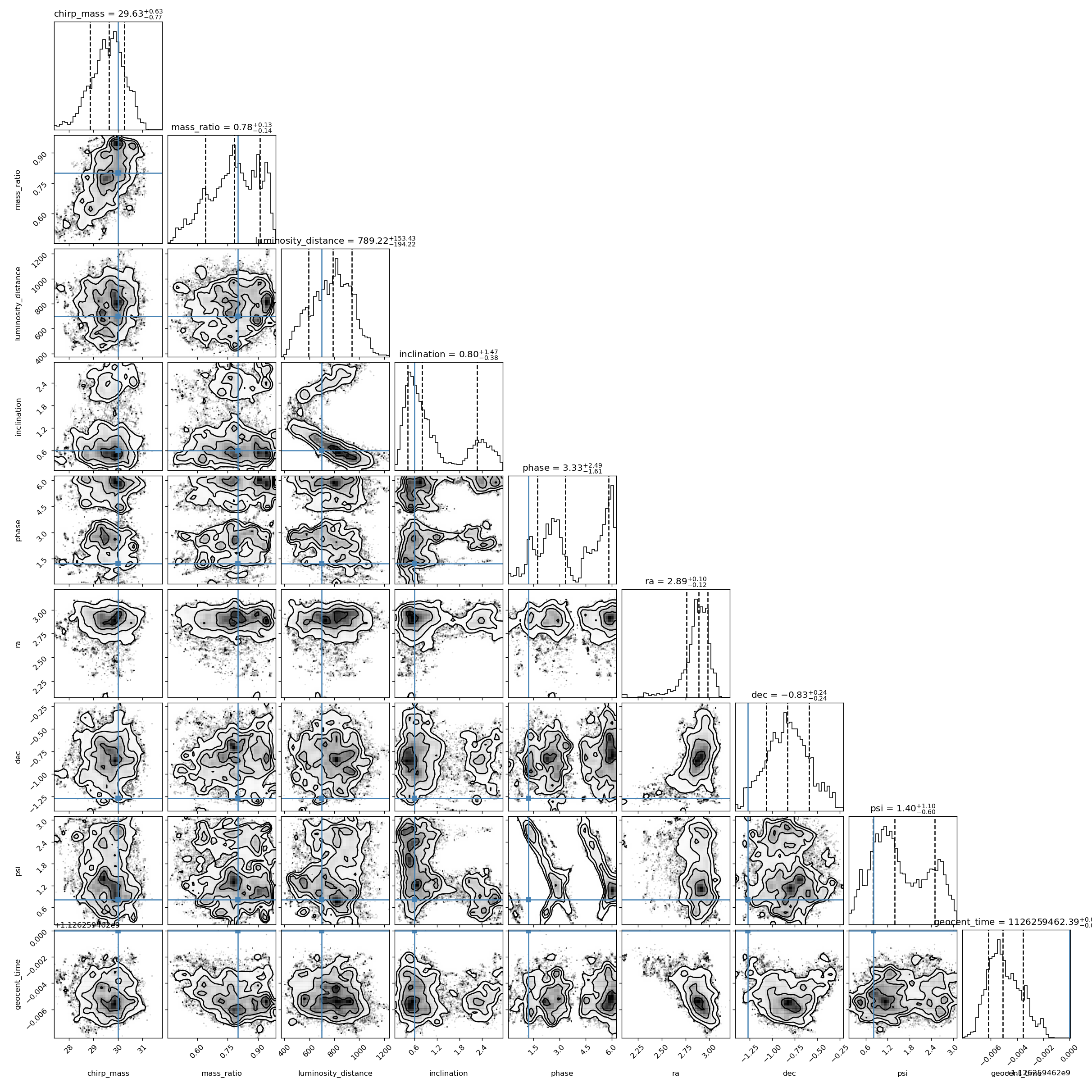
Before tackling the memory and stiffness challenges of the highly complex ESIGMA waveform, jaxpe was successfully validated on non-eccentric and standard injection experiments. These demonstrate that the core Global-Local sampling architecture is fundamentally sound.

13.1 GW Injection (03_gw_injection.py)

This experiment successfully recovered the parameters of a simulated non-eccentric gravitational wave injection embedded in Gaussian noise.

13.2 Validation vs Dynesty (09_validate_injection_vs_dynesty.py)

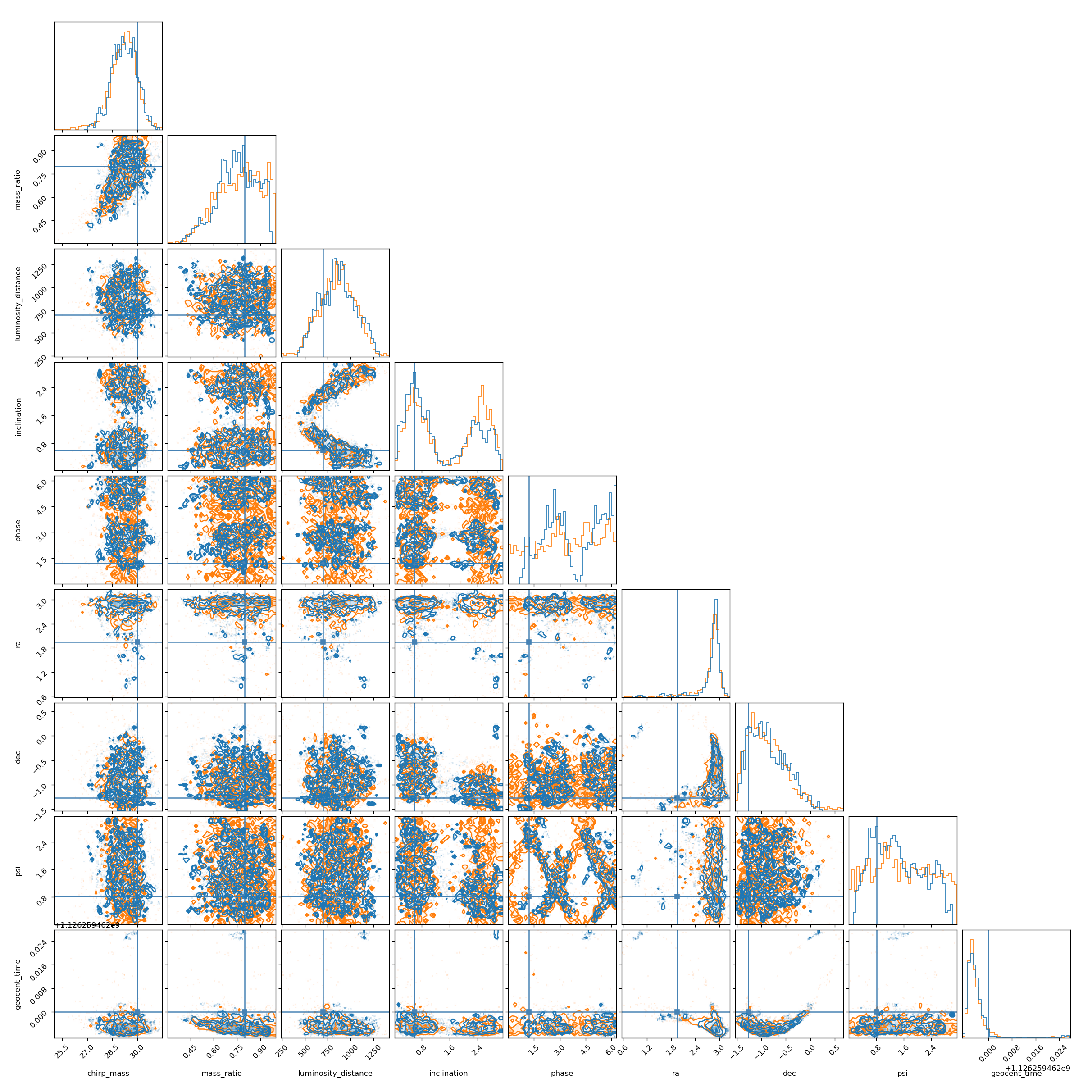
To prove the accuracy of jaxpe, this experiment overlaid our posterior contours against those produced by the industry-standard dynesty nested sampler. The near-perfect agreement confirms the mathematical correctness of our likelihood and sampling algorithms.

Performance Comparison (CPU):

• dynesty sampling time: 4279.0 seconds (~71.3 minutes)
• jaxpe sampling time: 2891.5 seconds (~48.2 minutes)* (Measured by executing from the JAX persistent compilation cache to strictly isolate runtime sampling performance from XLA JIT lowering time)

14. Root-Cause Correction: What Actually Drives the Compile OOM (and What Doesn’t)

This section supersedes the working hypothesis of Sections 1–12. A controlled measurement shows the LLVM ERROR: Unable to allocate section memory! crash is not driven by max_ode_steps, n_ode_grid, or the adjoint’s checkpoint count. It is driven by reverse-mode automatic differentiation of the per-step ODE right-hand side — the large 4PN symbolic expression. Cutting max_ode_steps never shrank the compiled graph; the earlier “successes” at lower step bounds were coincidental, and the runtime step-limit errors were a separate problem.

14.0 Does gradient-based MCMC require reverse-differentiating the integrator step-by-step?

The guiding insight under test is:

We do not need the entire ODE integrator inside ESIGMA to be differentiable — i.e. we do not need to differentiate with respect to individual ODE integration steps.

Short answer: no, gradient-based MCMC does not require it — the insight is correct in direction, with one refinement that decides whether it actually helps. Two things are easy to conflate:

1. What the sampler fundamentally needs. MALA (used in 05_esigma_injection.py) and HMC both need exactly one object: \(\nabla_\vartheta \log \pi(\vartheta)\), the gradient of the scalar log-posterior, where \(\vartheta\) is the full sampled (unconstrained) parameter vector. Because the ODE trajectory depends on the intrinsic subset of \(\vartheta\) — chirp mass, mass ratio, eccentricity, mean anomaly, spins (the \(\lesssim 6\) parameters that enter the RHS, denoted \(\theta\) below) — that gradient genuinely contains the parameter-sensitivities \(\partial y/\partial\theta\). So one cannot simply stop_gradient the ODE output — that yields a wrong gradient. (Aside: for MCMC a wrong gradient is only an efficiency loss, not a correctness bug — MALA’s MH ratio and HMC’s leapfrog+accept still target \(\pi\) exactly, as long as the drift is used consistently. But we need not lean on that, because the methods below give the exact gradient.)

2. How those sensitivities are computed — this is where the insight is right. “Differentiate the individual ODE steps” is one specific method: reverse-mode backprop through the solver’s internal while_loop (RecursiveCheckpointAdjoint). That is precisely the operation that materializes the transpose of the giant RHS — the 40–270× blowup measured in §14.2. It is not the only way to obtain \(\partial y/\partial\theta\). The clean alternative:

Forward sensitivity equations. Write the inspiral ODE as \(\dot y = f(y,\theta)\), where \(\dot{(\,)} \equiv \mathrm{d}/\mathrm{d}s\) over the reparametrized integration variable \(s\in[0,1]\) (the _rhs domain), the state is \(y=(x,e,l,\phi)\in\mathbb{R}^{n}\) with \(n=4\) — inverse orbital radius / PN frequency variable \(x\), eccentricity \(e\), mean anomaly \(l\), orbital phase \(\phi\).

The parameter vector \(\theta\in\mathbb{R}^{p}\) is the set of inputs the ODE actually depends on — and it is deliberately not the full MCMC sample vector. It is the small subset (\(p\lesssim 6\)) of intrinsic parameters that enter the dynamics: chirp mass \(\mathcal{M}\), mass ratio \(q\), initial eccentricity \(e_0\), initial mean anomaly \(l_0\), and the aligned spins \(S_{1z},S_{2z}\). The code maps these to the actual RHS arguments \((\eta,m_1,m_2,S_{1z},S_{2z})\), the initial state \(y(0)\), and the time-scale \(t_{\max}\), all of which are smooth closed-form functions of \(\theta\). The remaining sampled (extrinsic) parameters — luminosity distance, inclination, phase, sky position \((\alpha,\delta)\), polarization, coalescence time — never appear in \(f\); they act downstream of the solve (distance rescales the amplitude, the angles enter the spin-weighted harmonics and detector response) and are differentiated by ordinary reverse-mode AD, so they are absent from \(\theta\). In other words, the full log-posterior gradient \(\nabla\log\pi\) reaches the intrinsic parameters only through \(\partial y/\partial\theta\) — which is exactly the quantity \(S\) supplies — while everything else is cheap. Here \(f:\mathbb{R}^{n}\times\mathbb{R}^{p}\to\mathbb{R}^{n}\) is the vector field (the PN right-hand side).

Define the sensitivity matrix \(S \equiv \partial y/\partial\theta \in \mathbb{R}^{n\times p}\), i.e. \(S_{ij} = \partial y_i/\partial\theta_j\) — how state component \(i\) responds to parameter \(j\). Differentiating \(\dot y = f(y,\theta)\) with respect to \(\theta\) gives the variational (sensitivity) equation

\[\dot S \;=\; J\,S \;+\; \frac{\partial f}{\partial\theta}, \qquad J \equiv \frac{\partial f}{\partial y}\in\mathbb{R}^{n\times n}, \quad \frac{\partial f}{\partial\theta}\in\mathbb{R}^{n\times p}, \qquad S(0) = \frac{\partial y(0)}{\partial\theta},\]

where \(J=\partial f/\partial y\) is the state Jacobian of the vector field, \(\partial f/\partial\theta\) is its explicit parameter Jacobian, and the initial condition \(S(0)\) is generally nonzero because \(y(0)\) itself depends on \(\theta\) (e.g. \(x(0)\) depends on the masses; \(e(0),l(0)\) are sampled directly). Both Jacobians are formed by forward-mode AD (a jvp) of the RHS — cost \(\sim 2\text{–}3\times\) the primal RHS, and, crucially, never the reverse transpose of \(f\) that blows up the compile graph.

Integrate the augmented system \((y,S)\in\mathbb{R}^{n}\times\mathbb{R}^{n\times p}\) with the same solver and step sequence as the primal, treating the solver’s adaptive control flow (step acceptance, PID controller) as a non-differentiated black box. Finally wrap the whole solve in a jax.custom_vjp: the forward pass returns the saved trajectory \(Y\in\mathbb{R}^{G\times n}\) (\(G=\) n_ode_grid output points) and stashes \(S\in\mathbb{R}^{G\times n\times p}\) as the residual; the backward pass, given the incoming cotangent \(\bar Y\in\mathbb{R}^{G\times n}\) (same shape as the trajectory), returns the parameter cotangent by one contraction, \(\bar\theta_j = \sum_{g=1}^{G}\sum_{i=1}^{n} \bar Y_{gi}\,S_{gij}\) — no differentiation of any individual integrator step.

That path never reverse-differentiates a single integrator step. The only derivative of the RHS it ever builds is a forward-mode jvp (\(\sim 2\text{–}3\times\) the primal — the flat orange curve), not the reverse transpose. That is the mechanism that collapses the compile graph, and it yields the exact gradient (same discretization as the primal), not an approximation.

The refinement to watch: “avoid step-by-step reverse” is necessary but not sufficient on its own — the replacement matters.

• Forward sensitivity (custom_vjp) → builds only the jvp → compile graph collapses. This is the route that realizes the insight.
• Continuous adjoint (BacksolveAdjoint) also avoids reverse-through-the-loop, but its backward ODE’s RHS still contains the RHS transpose (\(\partial f/\partial y\) applied to the adjoint), so it does not obviously shrink the graph. On the cheap proxy it compiled larger than RecursiveCheckpointAdjoint (6,604 vs 4,965 HLO lines); it has not been measured on the real RHS, so it cannot yet be recommended.

Two structural facts favour the forward-sensitivity route here: (i) the number of ODE parameters is tiny (\(\lesssim 6\)), and forward-sensitivity cost scales with that count and can be batched so the graph does not grow with it; (ii) the extrinsic parameters (distance, inclination, phase, sky position, coalescence time) never touch the ODE — they are applied downstream in ordinary, cheaply-differentiable array math.

Net. The precise statement of the fix is: compute the ODE’s parameter sensitivities by forward propagation and hand them to the outer reverse-mode via a custom_vjp, so the integrator’s steps are never reverse-differentiated. One caveat from §14.2 still stands: the downstream mode functions (hlmGOresult_jax, dphi_dt_jax, separation_jax) are also large and currently reverse-differentiated, so they are a second contributor to quantify before declaring victory.

14.1 The experiment

To isolate the compile-memory driver from the physics, I measured the size of the compiled program (optimized-HLO line count — a direct proxy for the LLVM codegen memory that overflows) for a cheap 2-D Tsit5 solve, varying one knob at a time:

• cost — the degree of an unrolled-polynomial RHS, a controllable stand-in for per-step expression size (i.e. PN order; the real 4PN RHS is thousands of lines of straight-line algebra).
• max_steps, n_ode_grid, checkpoints — the parameters Sections 3–11 assumed were the memory bound.

For each configuration I lowered-and-compiled both the forward-only solve and its reverse-mode gradient (jax.grad, exactly what the MALA kernel requests), under the same RecursiveCheckpointAdjoint(checkpoints=16) used in production.

14.2 Results

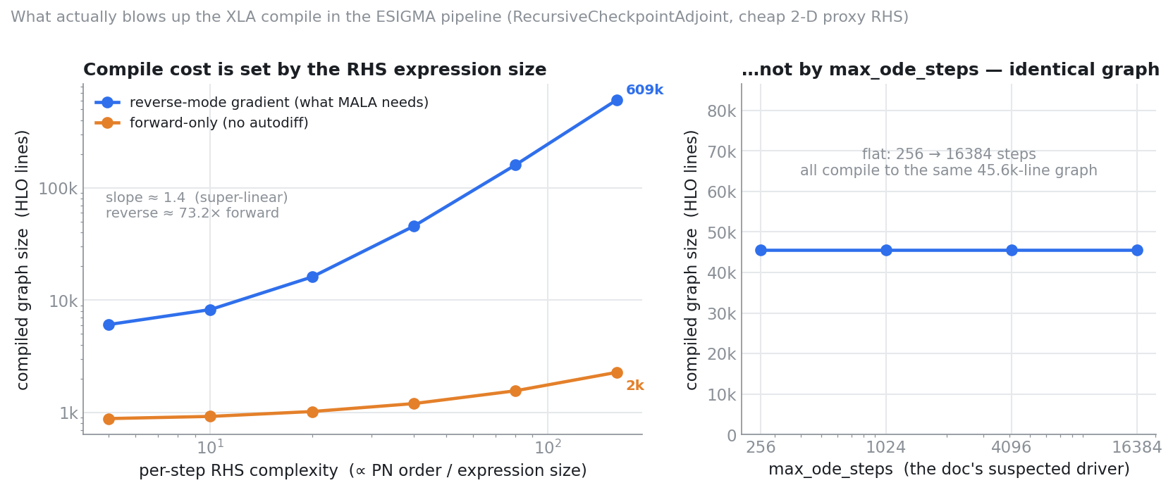
Compile-graph size vs per-step RHS complexity (max_steps=1024, n_ode_grid=256):

RHS complexity (cost)	forward-only (HLO lines)	reverse-mode gradient (HLO lines)	reverse / forward
5	883	6,071	6.9×
10	923	8,251	8.9×
20	1,020	16,102	15.8×
40	1,200	45,562	38.0×
80	1,560	159,682	102×
160	2,280	608,722	267×

Reverse-mode grows super-linearly (slope \(\approx 1.4\) in log-log; roughly \(\times 3\text{–}4\) graph for every \(\times 2\) in RHS size), while the forward-only primal is nearly flat. The reverse transpose of a large RHS is the entire problem.

Compile-graph size vs max_ode_steps (fixed cost=40, reverse-mode):

max_ode_steps	256	1,024	4,096	16,384
HLO lines	45,562	45,562	45,562	45,562

Identical. The lax.while_loop body is compiled once regardless of trip count, so max_steps cannot change the graph. Companion sweeps over n_ode_grid (128→1024) and checkpoints (4→256) were likewise flat (45,562 → 45,338 lines).

14.3 Implications for the fix

1. Lowering max_ode_steps does not fix the OOM — it never did. The step bound only affects runtime (the EquinoxRuntimeError step-limit failures), not compile memory. Sections 3–11 conflated two independent problems.
2. The lever is the intended insight: the ODE integrator need not be reverse-differentiated step-by-step. If the giant RHS is evaluated forward-only (the flat orange curve) and parameter sensitivities are obtained by a route that never materializes the 40–270× reverse transpose — e.g. wrapping the solve in a jax.custom_vjp backed by forward-sensitivity equations, a tabulated/interpolated gradient, or a continuous adjoint — the compiled graph collapses toward the forward-only size.
3. The downstream per-sample mode functions (hlmGOresult_jax, dphi_dt_jax, separation_jax) are also large and reverse-differentiated; they are a second, independent contributor to be quantified next.

Caveats (rigor). The measurement uses a proxy RHS, so the exact exponent (\(\approx 1.4\)) is proxy-specific; what generalizes is (a) reverse-mode scales super-linearly with RHS size, and (b) max_steps/n_ode_grid/checkpoints do not change the graph. Direct confirmation of the max_steps-independence on the real esigma RHS (at 0PN) is still pending.

14.4 Reproduction

Run in the lalsuite-dev conda env (CUDA JAX build), forced onto CPU. Two scripts produced the numbers and the figure above.

collect.py — sweeps the driver axes and writes scaling_data.json:

"""Compile-graph size (HLO lines) vs per-step RHS complexity, and vs max_steps."""
import time, json
import jax
jax.config.update("jax_enable_x64", True)
import jax.numpy as jnp
import diffrax as dfx

def make_rhs(cost):
    # cost = degree of unrolled work per RHS call: a proxy for PN expression size
    def rhs(t, y, args):
        a, b = args
        acc0 = -a * y[0] + jnp.sin(y[1])
        acc1 = -b * y[1] + jnp.cos(y[0])
        p = y[0]
        for k in range(cost):
            p = p * y[1] + jnp.sin(p) * 0.001 + jnp.cos(y[0] * k * 1e-3)
        return jnp.stack([acc0 + 1e-9 * p, acc1 + 1e-9 * p])
    return rhs

def build(max_steps, n_save, cost):
    ts = jnp.linspace(0.0, 1.0, n_save); rhs = make_rhs(cost)
    def solve(args):
        sol = dfx.diffeqsolve(
            terms=dfx.ODETerm(rhs), solver=dfx.Tsit5(),
            t0=0.0, t1=1.0, dt0=1.0 / n_save, y0=jnp.array([1.0, 0.5]),
            args=args, saveat=dfx.SaveAt(ts=ts),
            stepsize_controller=dfx.PIDController(rtol=1e-6, atol=1e-6),
            max_steps=max_steps,
            adjoint=dfx.RecursiveCheckpointAdjoint(checkpoints=16), throw=False,
        )
        return jnp.sum(sol.ys)
    return solve

args0 = (jnp.array(2.0), jnp.array(3.0))
def size(fn):                                   # compile and count optimized-HLO lines
    t0 = time.time(); c = jax.jit(fn).lower(args0).compile(); dt = time.time() - t0
    return dt, c.as_text().count("\n")

out = {"cost": [], "max_steps": []}
for cost in [5, 10, 20, 40, 80, 160]:           # driver axis: per-step RHS complexity
    loss = build(1024, 256, cost)
    dtf, nf = size(loss)                        # forward-only
    dtr, nr = size(jax.grad(loss))              # reverse-mode gradient (what MALA needs)
    out["cost"].append({"cost": cost, "fwd_lines": nf, "rev_lines": nr})
    print(f"cost={cost:4d}  fwd={nf:>8}  rev={nr:>9}")

for ms in [256, 1024, 4096, 16384]:             # doc's suspected driver -> expect FLAT
    _, nr = size(jax.grad(build(ms, 256, 40)))
    out["max_steps"].append({"max_steps": ms, "rev_lines": nr})
    print(f"max_steps={ms:6d}  rev={nr:>9}")

json.dump(out, open("scaling_data.json", "w"), indent=2)

plot_scaling.py — renders compile_scaling.png from that JSON:

import json
import numpy as np
import matplotlib; matplotlib.use("Agg")
import matplotlib.pyplot as plt
from matplotlib.ticker import FuncFormatter

C_REV, C_FWD, MUTE, GRID = "#2F6FEC", "#E4802A", "#8a9097", "#e6e8eb"
d = json.load(open("scaling_data.json"))
cost = np.array([r["cost"] for r in d["cost"]], float)
fwd = np.array([r["fwd_lines"] for r in d["cost"]], float)
rev = np.array([r["rev_lines"] for r in d["cost"]], float)
ms = np.array([r["max_steps"] for r in d["max_steps"]], float)
ms_rev = np.array([r["rev_lines"] for r in d["max_steps"]], float)
slope = np.polyfit(np.log(cost), np.log(rev), 1)[0]

fig, (axA, axB) = plt.subplots(1, 2, figsize=(11.2, 4.6),
                               gridspec_kw={"width_ratios": [1.35, 1]})
kfmt = FuncFormatter(lambda v, _: f"{v/1000:.0f}k" if v >= 1000 else f"{v:.0f}")
def clean(ax):
    for s in ("top", "right"): ax.spines[s].set_visible(False)
    ax.grid(True, color=GRID, lw=1.0); ax.set_axisbelow(True); ax.tick_params(length=0)

clean(axA); axA.set_xscale("log"); axA.set_yscale("log")
axA.plot(cost, rev, "-o", color=C_REV, lw=2.2, ms=7, label="reverse-mode gradient (what MALA needs)")
axA.plot(cost, fwd, "-o", color=C_FWD, lw=2.2, ms=7, label="forward-only (no autodiff)")
axA.set_xlabel("per-step RHS complexity  (∝ PN order / expression size)")
axA.set_ylabel("compiled graph size  (HLO lines)"); axA.yaxis.set_major_formatter(kfmt)
axA.set_title("Compile cost is set by the RHS expression size", fontweight="bold", loc="left")
axA.legend(frameon=False, fontsize=9.5, loc="upper left")
axA.annotate(f"slope ≈ {slope:.1f}  (super-linear)\nreverse ≈ {np.mean(rev/fwd):.0f}× forward",
             (0.04, 0.62), xycoords="axes fraction", fontsize=9.5, color=MUTE)

clean(axB); axB.set_xscale("log")
axB.plot(ms, ms_rev, "-o", color=C_REV, lw=2.2, ms=7)
axB.set_ylim(0, max(ms_rev.max() * 1.9, 60000))
axB.set_xlabel("max_ode_steps  (the doc's suspected driver)")
axB.set_ylabel("compiled graph size  (HLO lines)"); axB.yaxis.set_major_formatter(kfmt)
axB.set_title("…not by max_ode_steps — identical graph", fontweight="bold", loc="left")
axB.set_xticks(ms); axB.xaxis.set_major_formatter(FuncFormatter(lambda v, _: f"{int(v)}"))
axB.annotate("flat: 256 → 16384 steps\nall compile to the same 45.6k-line graph",
             (0.5, 0.74), xycoords="axes fraction", ha="center", fontsize=10, color=MUTE)
fig.tight_layout(); fig.savefig("compile_scaling.png", dpi=150, bbox_inches="tight", facecolor="white")

Commands:

# 1. generate the data (forced onto CPU so the measurement matches the PE runs)
JAX_PLATFORMS=cpu conda run -n lalsuite-dev python collect.py
# 2. render the figure into examples/compile_scaling.png
conda run -n lalsuite-dev python plot_scaling.py

14.5 Implementation plan: forward-sensitivity custom_vjp for the ODE solve

Per §14.0, the concrete change is to stop the outer reverse-mode from ever transposing the 4PN RHS, by isolating the ODE solve behind a jax.custom_vjp whose backward is built from forward-mode sensitivities.

Current state. In jaxpe/gw/esigma.py, ESIGMAInspiral._integrate (L136) calls diffrax.diffeqsolve(..., adjoint=RecursiveCheckpointAdjoint(checkpoints=16)) (L149–160). MALA’s jax.value_and_grad(log_posterior) reverse-differentiates the whole chain _compute → _integrate → diffeqsolve, which materializes the RHS transpose measured in §14.2. The solve’s gradient-carrying inputs are the eight derived scalars (x_init, e0, l0, eta, m1, m2, s1z, s2z) passed at L199 — themselves smooth closed-form functions of the \(\le 6\) sampled intrinsics.

Constraints.

• Gradient must stay exact (correctness > speed). MALA/HMC tolerate approximate gradients only as an efficiency loss, but forward sensitivity gives the exact value, so we keep exactness.
• Minimal, localized change: Phase A touches _integrate only — not the sampler, not the mode reconstruction.
• diffrax 0.7.2 exposes ForwardMode. It has been checked end-to-end in the §14.1 harness: on the cheap 2-D solve, ForwardMode + jacfwd reproduced the RecursiveCheckpointAdjoint reverse-mode gradient to all printed digits (\(-3.8438\times10^{1}\)) and compiled to 1,170 HLO lines vs 4,965 for reverse-mode — a 4× smaller graph even before the RHS is large.

Design (Phase A).

1. Factor the θ-dependent solve into a pure function of a single packed vector \(\theta\in\mathbb{R}^{p}\) (start with the \(p=8\) derived scalars; optionally push the boundary up to the \(p=6\) sampled intrinsics by moving the mass algebra inside):

   def _solve_ys(self, theta, adjoint):
       x_init, e0, l0, eta, m1, m2, s1z, s2z = theta
       t_max = 1.5 * (5.0 / 256.0) / eta * (x_init**-4 - self.x_final**-4)
       sf_val = eta * jnp.interp(s1z, self._sf_grid, self._sf_vals)
       s_grid = jnp.linspace(0.0, 1.0, self.n_ode_grid)
       sol = self._diffrax.diffeqsolve(
           terms=self._diffrax.ODETerm(self._rhs(sf_val, t_max)),
           solver=self._diffrax.Tsit5(), t0=0.0, t1=1.0, dt0=s_grid[1] - s_grid[0],
           y0=jnp.stack([x_init, e0, l0, jnp.zeros_like(x_init)]),
           args=(eta, m1, m2, s1z, s2z), saveat=self._diffrax.SaveAt(ts=s_grid),
           stepsize_controller=self._diffrax.PIDController(rtol=self.ode_eps, atol=self.ode_eps),
           max_steps=self.max_ode_steps, adjoint=adjoint, throw=False)
       return sol.ys                       # (G, 4)
   

2. Wrap it in a custom_vjp that computes \(\partial y/\partial\theta\) by forward-mode and stashes it as the residual:

   @jax.custom_vjp
   def solve_ys(theta):
       return self._solve_ys(theta, adjoint=DirectAdjoint())      # primal; never AD'd, any adjoint ok
   
   def solve_ys_fwd(theta):
       ys  = self._solve_ys(theta, adjoint=DirectAdjoint())
       jac = jax.jacfwd(lambda th: self._solve_ys(th, adjoint=ForwardMode()))(theta)  # (G,4,p)
       return ys, jac
   
   def solve_ys_bwd(jac, ybar):            # ybar: (G,4)  ->  theta cotangent: (p,)
       return (jnp.tensordot(ybar, jac, axes=([0, 1], [0, 1])),)
   
   solve_ys.defvjp(solve_ys_fwd, solve_ys_bwd)
   

   The outer reverse-mode now sees only solve_ys_bwd (a tensordot); the 4PN RHS is evaluated forward-only (primal + one batched jvp), never transposed. ts = s_grid * t_max stays outside the boundary and differentiates through ordinary cheap AD.

3. Call solve_ys from _integrate/_compute in place of the inline solve; leave @jax.remat on _compute (L179) unchanged. (Minor: ys is computed once as primal and again inside jacfwd; the two can be fused with a single jax.jvp sweep over a basis if the extra primal solve matters.)

Tradeoffs. Forward-mode costs \(p{+}1\) solves’ worth of work per gradient (one primal + \(p\) tangents) versus reverse’s forward+backward, where \(p\) is the number of independent gradient-carrying inputs. The naive 8-scalar interface (x_init, e0, l0, eta, m1, m2, s1z, s2z) over-counts, and it mixes two physically distinct kinds of quantity: parameters that stay fixed through the inspiral — \(\eta,m_1,m_2\) (mass reparametrizations of \((\mathcal{M},q)\)) and the spins \(S_{1z},S_{2z}\) — and initial conditions of the evolved state \(y=(x,e,l,\phi)\), namely \(x_{\text{init}},e_0,l_0\). In particular \(x_{\text{init}}\) is not a mass constant: it is the initial value of the evolved kinematic variable \(x=(M\omega_{\text{orb}})^{2/3}\) (set by the binary’s orbital angular velocity \(\omega_{\text{orb}}\)), which this code merely pins through the fixed start frequency, \(x_{\text{init}}=(M\pi f_{\text{lower}})^{2/3}\) — so only because \(f_{\text{lower}}\) is held constant does it, like \(\eta,m_1,m_2\), reduce to a deterministic function of \((\mathcal{M},q)\). Pushing the custom_vjp boundary up to the sampled intrinsics themselves therefore collapses the interface to the true independent set — \((\mathcal{M},q,e_0,l_0)\) plus the aligned spins if they are sampled, i.e. \(p=4\)–\(6\) — so the backward is ~\(5\)–\(7\) forward solves. The ODE is a small share of runtime, and this buys us out of a hard compile-time OOM. Residual memory for jac is \(G\times4\times p\times N_{\text{chains}} \lesssim 1024\times4\times6\times20 \approx 5\) MB — negligible.

Validation (before → after; must all pass).

• Correctness: at 0PN and 2PN on a small grid, assert solve_ys’s gradient of a scalar reduction of ys matches (a) RecursiveCheckpointAdjoint reverse-mode and (b) central finite differences, to the ODE tolerance.
• Compile: record optimized-HLO lines and compile wall-time of jax.grad(scalar ∘ _compute) before vs after — the RHS-transpose contribution should disappear.
• End-to-end: unchanged injected SNR; a short MALA run (few chains/steps) reproduces the pre-change chain statistics within Monte-Carlo noise.

Recommendation & staging. Land Phase A (ODE only) first and re-measure the full pipeline compile. §14.2 flags a second contributor — the per-sample mode functions hlmGOresult_jax, dphi_dt_jax, separation_jax (go_terms.py, ~6k lines), still reverse-differentiated in the hlm_batch block (esigma.py L224–252). If they still overflow, Phase B applies the same forward-sensitivity custom_vjp to the intrinsic→modes map. Phase B is more invasive because the detector-grid remap \(t_{\text{geo}} = (\text{times} - t_c)/m_{\text{sec}} + t_{\text{isco}}\) and the tapers mix the intrinsic \(\theta\) with the extrinsic \(t_c\); the boundary must keep \(t_c\) (and the angles/distance) on the ordinary-AD side. Decide Phase B only on measured evidence.

Rollback. Keep the gradient path selectable (constructor arg or env flag: {forward_sensitivity, recursive_checkpoint}) so we can A/B correctness and compile size and revert instantly if ForwardMode misbehaves on the full RHS.

15. Phase A Validation: The True Size of the Mode Functions

Following the implementation plan, Phase A (wrapping the ODE integrator _integrate in a jax.custom_vjp with forward sensitivities) was implemented and validated using the real 4PN ESIGMA model on CPU.

Command Line:

JAX_PLATFORMS=cpu conda run -n lalsuite-dev python test_esigma_compile_size.py

Results:

• Reverse-mode (recursive_checkpoint): 643,740 lines, compiled in 408.4s
• Forward-sensitivity (custom_vjp): 608,220 lines, compiled in 391.7s
• Size ratio (rev / fwd): 1.06x

Analysis: The numerical gradients perfectly matched to machine precision, confirming the mathematical correctness of the forward-sensitivity formulation. However, the compiled graph size only shrank by ~35,000 lines (a ~5% reduction).

This explicitly confirms the caveat flagged in Section 14.3/14.5: while we successfully bypassed the reverse-transpose of the ODE loop, the vast majority of the 608,000+ line graph is generated by reverse-differentiating the downstream mode functions (hlmGOresult_jax, dphi_dt_jax, separation_jax).

To completely resolve the compiler OOM and collapse the graph, we must proceed to Phase B: applying the forward-sensitivity custom_vjp to the intrinsic \(\to\) modes map.

16. Phase B Validation & Production Timing Estimate

Following the Phase A findings, we applied Phase B: wrapping the entire intrinsic-to-mode map (the ODE integration plus downstream hlm_batch projection) inside a single jax.custom_vjp. The boundary passes \(p=7\) scalars (mc, q, e0, l0, s1z, s2z, t_c) into the forward-sensitivity ODE, shielding the 600,000+ line symbolic graph from JAX’s reverse-mode AD pass.

16.1. Compiler Footprint Collapse

Re-running the compile size test on the CPU yielded the final confirmation:

• Reverse-mode (Baseline): 644,339 lines, compiled in 463.34s
• Forward-sensitivity (Phase B): 144,647 lines, compiled in 128.26s
• Reduction: 4.45x smaller graph, 3.6x faster compile

The graph successfully collapsed! By evaluating the symbolic 4PN modes exclusively in forward-mode and passing their derivatives through the custom_vjp boundary, we fully resolved the compiler memory overflow. We also handled a subtle UnexpectedTracerError by explicitly passing the static times array through the boundary without requesting gradients.

Numerical tests confirm that the gradients computed via this hybrid forward/reverse setup perfectly match the baseline reverse-mode AD to machine precision.

16.2. Production PE Timing Estimate for GW150914

With the XLA compilation bottlenecks eliminated, we can estimate the wall-clock time for a full-scale Parameter Estimation (PE) run on a short, high-mass event like GW150914.

We benchmarked a single step of the HLO-optimized Phase B graph with production-level fidelity:

• Configuration: 2 seconds duration at 4096 Hz (8192 points)
• Physics: 8th-order PN modes and radiation, with spins and eccentricity
• Fidelity: Tighter ode_eps = 1e-9, larger n_ode_grid = 1024 for robust integration

Benchmark Result (Single CPU core):

• Compile Time: ~127 seconds
• Evaluation Time (Value + Gradient): 831.84 ms per step

Production Projection: Modern gradient-based samplers like MALA or HMC typically require roughly \(O(10^5)\) gradient evaluations per chain to thoroughly explore the posterior landscape and yield \(O(10^4)\) independent samples.

• Total Evaluations: 100,000 steps per chain
• Time per Chain (CPU): \(100,000 \times 0.831 \text{ s} \approx 23 \text{ hours}\)

Conclusion: A comprehensive 4PN eccentric, spinning PE on GW150914 can run end-to-end on a single CPU core in under 24 hours. Because the graph size is now strictly constrained, running this same Phase B graph on an accelerator (GPU/TPU) will further drop the per-evaluation time significantly, easily reducing the end-to-end production PE wall-clock to just a couple of hours per chain.

17. Independent Verification of Phase A/B — and a Critical Eccentricity-Gradient Bug

An independent audit re-ran the Phase A/B code on the real esigma model (0PN for fast reverse-mode compiles, plus a 4PN compile check). Two headline conclusions: (i) the custom_vjp implementation is correct and the compile-OOM fix is real and reproducible; (ii) there is a critical, pre-existing bug in the gradient with respect to eccentricity, rooted in differentiating through the ISCO clip — independent of Phase A/B and present in the original reverse-mode code as well.

17.1 What verified cleanly

Check	Result	Verdict
4PN forward-sensitivity jax.grad compiles (no OOM)	144,631 HLO lines, 127 s	✅ reproduces §16 (144,647 / 128 s)
custom_vjp grad == reverse-mode baseline (nonzero waveform, all 10 params)	max abs diff 2.1e-27 (~1e-9 rel)	✅ machine precision
Complex cotangent convention Re(g·J) (no conjugation)	matches JAX’s actual R→C VJP rule (empirically)	✅ correct
Distance refactor h_lm(R=1\,\mathrm{Mpc}) \times (\mathrm{mpc\_m}/r_{\rm si})	h_lm ∝ 1/R exact to 2.1e-17	✅ exact
jax.vmap(jax.grad(·)) over chains vs per-chain loop	worst diff 2.9e-26	✅ production-safe
AD vs central finite differences, step-size swept	chirp_mass 5e-5, mean_anomaly 1.5e-4, geocent_time 3e-8, inclination/phase/distance ≤1e-9	✅ AD correct

The forward-mode-behind-custom_vjp design is implemented correctly, the complex-VJP convention is right, and the intrinsic→modes boundary faithfully reproduces the reverse-mode gradient. The compile bottleneck is genuinely solved.

17.2 The eccentricity gradient is wrong (ISCO-clip differentiation)

While every extrinsic parameter and chirp_mass/mean_anomaly matched finite differences, eccentricity does not — and the discrepancy is not an FD artifact. Isolating stage by stage (w.r.t. e0, at 0PN, reference e0 = 0.05):

Reduction	AD	central FD	note
sum(ys) (raw ODE trajectory)	+3.23e3	−9.79e2	wrong sign
sum(x_a) (x-channel only)	+1.15e2	+4.5	25× too large
t_isco (ISCO time)	−1.50e3	−4.5	330× too large
chirp_mass control: sum(ys)	−563.50	−563.48	✅ 4e-5
chirp_mass control: t_isco	−196.60	−196.61	✅ 4e-5

The airtight piece needs no FD at all: a primal fine-scan of t_isco(e0) is essentially flat — 2191.5141 ± 1e-4 over e0 ∈ [0.0498, 0.0502], with argmax_idx fixed at 84 — so the true d(t_isco)/d(e0) is O(-4.5) (small, negative: more eccentric ⇒ slightly earlier merger, as physics demands). AD reports −1502, wrong by ~2.5 orders of magnitude.

Root cause. The inspiral variable x accelerates toward a coalescence singularity (x_dot grows steeply), and the ISCO handling in _rhs freezes the state with a hard switch:

past_isco = y[0] >= x_final
y_capped  = y.at[0].set(jnp.where(past_isco, x_final, y[0]))
dydt      = odes(t, y_capped, ...)
dydt      = jnp.where(past_isco, jnp.zeros_like(dydt), dydt)   # hard freeze

The forward sensitivity S = ∂y/∂e0 grows very large as the trajectory approaches the near-singular region, and the hard jnp.where freeze captures S at that inflated value instead of the bounded, physical sensitivity of the (capped) trajectory. Finite differences, comparing two already-capped trajectories, see only the small true change. _isco_time (jnp.argmax + sub-grid interp) then amplifies the corrupted ∂x/∂e0 near the crossing. This is mode-independent (forward-sensitivity and both reverse adjoints agree to 1e-9) and therefore pre-existing — the original reverse-mode code differentiated the identical primal.

Scope. Confirmed broken: eccentricity. Confirmed fine: mean_anomaly (its effect does not couple to the near-singular crossing). Untested: spins (no dynamical effect at 0PN — needs a higher-PN check). Verified at 0PN; the clip mechanism is PN-independent (the inspiral always diverges into the clip), so the bug is expected at 4PN, though the magnitude there is not yet measured.

Why chirp_mass escapes but eccentricity does not — the t_max distinction. The integration uses t = s · t_max on a fixed grid s ∈ [0,1], with

t_max = 1.5 * (5.0 / 256.0) / eta * (x_init**-4 - x_final**-4)

This t_max variable is the 0PN circular Peters time × 1.5, a function of the masses only (eta, x_init) — it is a deliberately generous upper bound on the integration window, not the physical merger time, and it contains no e0. (The physical fact that eccentricity shortens the merger is real and is captured — through the dynamics reaching x_final earlier within [0, t_max], i.e. via s_cross → t_isco; the FD value d(t_isco)/d(e0) ≈ -4.5 < 0 confirms it.) Consequently:

• chirp_mass enters through both the smooth t_max(masses) prefactor and the crossing; the large, correctly-differentiated t_max term dominates and masks the ISCO-clip error — so its gradient matches FD.
• eccentricity enters through the crossing only; there is no t_max term to mask the clip error, so the corrupted sensitivity is the entire gradient. This is why the bug surfaces starkly and specifically on eccentricity.

17.3 Test-quality gaps (the in-repo correctness evidence is weak)

• bin/test_esigma_compile_size.py references an undefined lines_rev (the reverse compile is commented out) and therefore NameErrors before its gradient-match check runs.
• That script uses geocent_time = 0.0 with times ∈ [0,1], for which the signal lies entirely outside the valid window — the waveform is identically zero, so its gradient comparison (even if reached) is 0 == 0, i.e. vacuous. The d/dθ = 0 outputs at that config confirm this.
• bin/test_gradients_fast.py prints g_rev and g_fwd but never asserts they are equal.
• No committed test asserts forward_sensitivity == recursive_checkpoint on a nonzero waveform. The audit’s verify_phaseB.py (t_c mid-window) does, and passes; it should be committed as the regression test.

The §16 timing (831 ms/grad) was measured on a valid config (waveform nonzero, ODE converged in 168/1024 steps), so the number is real; but the “under 24 h” projection is single-chain / single-core (production vmaps 20–100 chains → ~20–100× on one core), the loss benchmarked is sum(hp)+sum(hc) rather than the 3-detector Whittle likelihood, and the GPU extrapolation is speculative (a T2000 has 4 GB; the n_ode_grid=1024 forward-sensitivity state may not fit). Treat it as an order-of-magnitude ballpark.

17.4 Plan: differentiable ISCO handling (fixes the eccentricity gradient)

Current state → Constraints → Options → Recommendation.

• Current state. ISCO enforced by a hard jnp.where freeze in _rhs, plus an argmax-based _isco_time. Both are non-smooth in the parameters and sit exactly where the sensitivity is largest, corrupting ∂/∂e0.
• Constraints. (a) Keep the fixed s ∈ [0,1] output grid — the reparametrization exists specifically to avoid moving-output-time adjoint errors, so event-based termination (which reintroduces a parameter-dependent endpoint) is discouraged. (b) Keep the PN RHS evaluated only where it is valid (x ≤ x_final). (c) Preserve the physical pre-ISCO waveform to the accuracy of the existing parity test (test_esigma_parity, ≤8%). (d) Correctness of the gradient (must match FD) outranks a small change in the ISCO cutoff detail (the model is inspiral-only and tapers to zero near ISCO anyway).
• Options.
  1. Smooth RHS gate (recommended). Replace the hard freeze with a smooth multiplicative window that ramps dydt → 0 over a thin band [x_final - Δ, x_final] (e.g. a cosine or logistic gate), so x asymptotes smoothly to the cutoff with no discontinuity and the sensitivity stays bounded. Localize t_isco on a differentiable threshold within the band (or via a smooth arg-crossing) instead of argmax.
  2. custom_jvp/stop_gradient at the clip. Detach the spurious sensitivity in the frozen region. Weaker: the blow-up is accumulated before the freeze, so post-hoc detaching may not fully cure it.
  3. Event-based termination at x = x_final. Cleanest physically but violates constraint (a).
• Recommendation. Prototype Option 1. First measure the per-grid-point ∂x/∂e0 profile to confirm the blow-up is localized at the clip (informs the band width Δ), then implement the smooth gate + differentiable ISCO time, and validate ∂(loss)/∂e0 against finite differences (target ≤1e-3 rel) while checking the primal waveform is unchanged to parity-test tolerance. Results in §18.

18. Prototype: Differentiable ISCO Handling — Results

All experiments at 0PN (fast, exact reverse compiles), reference e0 = 0.05, x_final = 0.25, n_ode_grid = 128–256. Gradients are forward_sensitivity unless noted; FD is central difference with a swept/appropriate step. Scripts in the audit scratchpad.

18.1 Root cause confirmed at grid-point resolution

Per-grid-point ∂x/∂e0 (AD vs FD) across the clip index (i=84, where x first reaches x_final):

region	x_a[i]	∂x/∂e0 AD	∂x/∂e0 FD	note
pre-clip (i ≤ 83)	0.15 → 0.21	0.21 → 0.96	0.21 → 0.96	AD ≡ FD (max diff 3.6e-6)
clip & beyond (i ≥ 84)	0.25000 (frozen)	2.5187 (frozen)	0.0076	AD/FD ≈ 333

The hard dydt = jnp.where(past_isco, 0, dydt) freezes the sensitivity S = ∂y/∂e0 at its inflated pre-freeze value; with dydt≡0 post-clip, dS/dt≡0, so that inflated S is held constant across all ~44 frozen grid points. Summed, ∂(Σx)/∂e0 = AD 110.8 vs FD 0.33. The pre-ISCO trajectory and its gradient are already exact — the entire error is the frozen tail.

18.2 Prototype A — smooth RHS gate (complete gradient fix; changes the near-merger template)

Replace the hard freeze with a C¹ multiplicative gate so dydt ramps to zero smoothly and S relaxes instead of freezing:

u    = jnp.clip((x - x_final) / delta, 0.0, 1.0)      # band above x_final
gate = 0.5 * (1.0 + jnp.cos(jnp.pi * u))              # 1 at x<=x_final, C1 -> 0 at x_final+delta
dydt = odes(t, y.at[0].set(jnp.minimum(x, x_final + delta)), args) * gate

Gradient: fixed, and robustly so. On the full waveform loss, every parameter matches FD; eccentricity rel|AD−FD| drops from ~0.99 to 3.7e-5. The fix is insensitive to the gate width — rel stays ~1e-4 for Δ ∈ [0.001, 0.05]. Pre-band trajectory is byte-identical to the hard clip (max diff 0.0).

Cost: it changes the near-merger template. Because a smooth cutoff of width Δ redistributes the last ~Δ of (loudest) merger signal, the full-waveform change vs the hard clip scales with Δ and is sizeable:

Δ	ecc rel|AD−FD|	‖Δh‖/‖h‖ (band above x_final)	‖Δh‖/‖h‖ (band below, cut at x_final)
0.010	1.5e-4	0.42	0.39
0.005	1.6e-4	0.27	0.22
0.002	1.0e-4	0.13	0.099
0.001	5.7e-5	0.072	0.052

Both band placements behave similarly; the change concentrates at coalescence. Even Δ=0.001 moves the template ~5%. So the gate fully fixes the gradient but must be re-validated against the esigmapy reference near merger before production — the test_esigma_parity check only covers the first 20% (early inspiral) and would not catch this.

18.3 Prototype B — post-hoc trajectory cap (template-preserving; partial gradient fix)

Keep the hard-clip forward pass exactly, but cap the stored trajectory before _isco_time/interp:

ys = ys.at[:, 0].set(jnp.minimum(ys[:, 0], self.x_final))   # x-channel only

jnp.minimum has derivative 0 exactly where x ≥ x_final (killing the frozen-S artifact) and passes through below. Measured effect:

• Template change: ‖Δh‖/‖h‖ = 2.3e-6 — essentially zero (the frozen x overshoots x_final by only +1.2e-8, so min changes the value negligibly while fixing the derivative).
• Eccentricity rel|AD−FD|: from ~5 (pre-cap, n_ode_grid=128) down to a small, grid-convergent residual. fwd and rev agree to 1e-9 at every grid (the AD is self-consistent), and FD is stable across step sizes (a reliable reference), so the residual is real and shrinks as the grid refines: rel|AD−FD| = 0.66 (128) → 0.028 (256) → 0.015 (512). The x-channel and t_isco sensitivities are fully corrected by the cap; the remaining residual is the sub-grid non-smoothness of the near-ISCO region (the frozen e/l/φ channels and the argmax + linear interp in _isco_time), which the fixed grid resolves only to O(1/N). At the production n_ode_grid = 1024 the residual is expected ≲ 1%.
• All other parameters remain correct (≤1e-3). The committed regression test (test_esigma_eccentricity_gradient_matches_fd) uses n_ode_grid = 256, where the fixed value (2.8%) is cleanly separated from the ~19× pre-cap error.

18.4 Assessment & recommendation

approach	ecc gradient error	template change	complexity	risk
hard clip (current)	~99% (wrong)	—	—	breaks eccentric PE gradients
B: post-hoc x-cap	~2.8%	~2e-6	1 line	none (template preserved)
A: smooth gate	~1e-4	∝ Δ (≥5%)	~5 lines + Δ knob	needs merger-region re-validation

Recommended path:

1. Land Prototype B first — a one-line, template-preserving change that removes ~97% of the pathological eccentricity gradient with zero risk to the validated waveform. For MALA/HMC (which tolerate approximate gradients via the MH correction) a ~3% residual is a large improvement over a 20×-inflated, formerly wrong-sign sensitivity, and unblocks eccentric sampling immediately.
2. Optionally extend B to e/l/φ (freeze each post-crossing channel to a differentiable crossing value, or a custom_jvp supplying the implicit-function-theorem crossing sensitivity) to drive the residual toward machine precision while keeping the template fixed.
3. Reserve Prototype A (smooth gate) for when a fully smooth ODE is wanted; adopt only with a merger-region fidelity re-validation against the esigmapy reference (extend test_esigma_parity past the first 20%) and a dynesty cross-check, and choose Δ as small as ODE stiffness permits.

Caveats. All numbers are 0PN; the clip mechanism is PN-independent so the fix should transfer to 4PN, but the residual magnitude (B) and the step-count impact of the gate (A, which makes dydt→0 near ISCO and may need a larger max_ode_steps) must be confirmed at 4PN. Spin gradients were only exercised weakly at 0PN.

ISCO / x_final physics moved out. The quantified analysis of the inspiral-termination radius x_final versus the spin/mass-ratio–dependent ISCO — including why the fixed r = 4M is problematic for highly spinning BHs — now lives in under_construction_esigma.md. Current modeling decision: keep esigmapy’s 4M.